
Asset returns#
Let \(P_t\) be the price of an asset at time \(t\). We’ll define the gross return on the asset over one period as
where \(D_t\) denotes the value of any dividends paid during the period.
The net return is simply
The first term is the capital gains yield and the second is the dividend yield.
import wrds

db = wrds.Connection()
Loading library list...
Done
As an example, we’ll work with some historical price data for Apple.
sql = """
    SELECT dlycaldt, dlyprc, dlyret, dlyretx
    FROM crsp.dsf_v2
    WHERE permno = 14593
    AND dlycaldt >= '01/01/2019' AND dlycaldt <= '12/31/2020'
"""

aapl = db.raw_sql(sql, date_cols=['dlycaldt'])

aapl = (aapl
        .rename(columns={'dlycaldt': 'date', 'dlyprc': 'prc', 'dlyret': 'ret', 'dlyretx': 'retx'})
        .set_index('date')
        .sort_index())
aapl.loc['2020-08']
| prc | ret | retx | |
|---|---|---|---|
| date | |||
| 2020-08-03 | 435.75 | 0.025198 | 0.025198 |
| 2020-08-04 | 438.66 | 0.006678 | 0.006678 |
| 2020-08-05 | 440.25 | 0.003625 | 0.003625 |
| 2020-08-06 | 455.61 | 0.034889 | 0.034889 |
| 2020-08-07 | 444.45 | -0.022695 | -0.024495 |
| 2020-08-10 | 450.91 | 0.014535 | 0.014535 |
| 2020-08-11 | 437.50 | -0.029740 | -0.029740 |
| 2020-08-12 | 452.04 | 0.033234 | 0.033234 |
| 2020-08-13 | 460.04 | 0.017698 | 0.017698 |
| 2020-08-14 | 459.63 | -0.000891 | -0.000891 |
| 2020-08-17 | 458.43 | -0.002611 | -0.002611 |
| 2020-08-18 | 462.25 | 0.008333 | 0.008333 |
| 2020-08-19 | 462.83 | 0.001255 | 0.001255 |
| 2020-08-20 | 473.10 | 0.022190 | 0.022190 |
| 2020-08-21 | 497.48 | 0.051532 | 0.051532 |
| 2020-08-24 | 503.43 | 0.011960 | 0.011960 |
| 2020-08-25 | 499.30 | -0.008204 | -0.008204 |
| 2020-08-26 | 506.09 | 0.013599 | 0.013599 |
| 2020-08-27 | 500.04 | -0.011954 | -0.011954 |
| 2020-08-28 | 499.23 | -0.001620 | -0.001620 |
| 2020-08-31 | 129.04 | 0.033912 | 0.033912 |
CRSP provides two return variables:
retis the total return, \(R_t\);retxexcludes the dividend (i.e. it is the capital gains yield).
Note
CRSP makes data available in both daily and monthly files. Variables in the daily file are often prepended with dly and those in the monthly file with mth. So the date in one file is dlycaldt while in the other it’s mthcaldt. Similarly, we have dlyret and mthret, and so on.
Notice that
so we can recover the dividend from the difference in these two series by multiplying by the lagged price. And, obviously, if the dividend is zero the two returns will be identical.
divs = (aapl['ret'] - aapl['retx']) * aapl['prc'].shift()

divs[divs>0].round(3)
date
2019-02-08    0.730
2019-05-10    0.770
2019-08-09    0.770
2019-11-07    0.770
2020-02-07    0.770
2020-05-08    0.820
2020-08-07    0.820
2020-11-06    0.205
dtype: float64
db.raw_sql("""
           SELECT disexdt, disdivamt, disdeclaredt, disrecorddt, dispaydt
           FROM crsp.stkdistributions
           WHERE permno = 14593 AND disordinaryflg = 'Y'
           AND disexdt >= '01/01/2019' AND disexdt <= '12/31/2020'
           """,
           date_cols=['disexdt', 'disdeclaredt', 'disrecorddt', 'dispaydt'])
| disexdt | disdivamt | disdeclaredt | disrecorddt | dispaydt | |
|---|---|---|---|---|---|
| 0 | 2019-02-08 | 0.730 | 2019-01-29 | 2019-02-11 | 2019-02-14 |
| 1 | 2019-05-10 | 0.770 | 2019-04-30 | 2019-05-13 | 2019-05-16 |
| 2 | 2019-08-09 | 0.770 | 2019-07-30 | 2019-08-12 | 2019-08-15 |
| 3 | 2019-11-07 | 0.770 | 2019-10-30 | 2019-11-11 | 2019-11-14 |
| 4 | 2020-02-07 | 0.770 | 2020-01-28 | 2020-02-10 | 2020-02-13 |
| 5 | 2020-05-08 | 0.820 | 2020-04-30 | 2020-05-11 | 2020-05-14 |
| 6 | 2020-08-07 | 0.820 | 2020-07-30 | 2020-08-10 | 2020-08-13 |
| 7 | 2020-11-06 | 0.205 | 2020-10-29 | 2020-11-09 | 2020-11-12 |
Compound returns#
Holding the asset for \(k\) periods would earn a gross return of
That is, the \(k\)-period return is simply the product of the \(k\) one-period returns; for this reason it is also called the compound return.
Assets may generate a return that is compounded over varying intervals. For example, an asset generating a return per year of \(R\) but compouning \(n\) times per year will have a total return of
R = 0.1

prds = [1, 2, 4, 12, 52, 365, 24*365]
vals = [(1+R/n)**n for n in prds]

tbl = pd.DataFrame(vals, index=prds, columns=['Gross return'])
tbl.index.name = 'Frequency'

tbl
| Gross return | |
|---|---|
| Frequency | |
| 1 | 1.100000 |
| 2 | 1.102500 |
| 4 | 1.103813 |
| 12 | 1.104713 |
| 52 | 1.105065 |
| 365 | 1.105156 |
| 8760 | 1.105170 |
In the limit this leads to a continuous compounding,
With continuous compounding, the asset value after one year is
np.exp(0.1)
np.float64(1.1051709180756477)
Log returns#
The log return, or continuously compounded return is
where \(\Delta x_t := x_t - x_{t-1}\) is the difference operator.
The multiperiod log return is simply the sum of the continuously compounded one-period returns.
Using the first-order Taylor expansion of \(\ln(1+x)\) we can see that
so, for small returns, the log return will be close to the net return; this similarity breaks down as price changes become larger.
Exercise
Calculate the log return using Apple’s returns. On what dates is the difference between the log return and the standard return greater than 0.005?
Solution
aapl['logret'] = np.log(1+aapl['ret'])

# create a "mask" of Boolean values to select rows
mask = (aapl['logret'] - aapl['ret']).abs() > 0.005

aapl[mask]
We can see that the returns differ on days when Apple’s return is either very high or very low bigger than about 9% in absolute value.
Aggregating returns#
aapl.resample('ME')['logret'].sum().head()
date
2019-01-31    0.053687
2019-02-28    0.043799
2019-03-31    0.092601
2019-04-30    0.054900
2019-05-31   -0.132581
Freq: ME, Name: logret, dtype: float64
aapl.resample('ME')['ret'].apply(lambda x: (1+x).product()-1).head()
date
2019-01-31    0.055154
2019-02-28    0.044772
2019-03-31    0.097024
2019-04-30    0.056435
2019-05-31   -0.124168
Freq: ME, Name: ret, dtype: float64
We can compare these to the monthly return data in CRSP.
db.raw_sql("""
    SELECT mthcaldt, mthprc, mthret, mthretx
    FROM crsp.msf_v2
    WHERE permno = 14593
    AND mthcaldt >= '01/01/2019' AND mthcaldt <= '06/30/2019'
""")
| mthcaldt | mthprc | mthret | mthretx | |
|---|---|---|---|---|
| 0 | 2019-01-31 | 166.44 | 0.055154 | 0.055154 |
| 1 | 2019-02-28 | 173.15 | 0.044771 | 0.040315 |
| 2 | 2019-03-29 | 189.95 | 0.097026 | 0.097026 |
| 3 | 2019-04-30 | 200.67 | 0.056436 | 0.056436 |
| 4 | 2019-05-31 | 175.07 | -0.124166 | -0.127573 |
| 5 | 2019-06-28 | 197.92 | 0.130519 | 0.130519 |
When we resample, we can aggregate data with numerous arbitrary functions.
# quarterly return statistics

aapl.resample('QE')['ret'].agg(['mean', 'std', 'min', 'max'])
| mean | std | min | max | |
|---|---|---|---|---|
| date | ||||
| 2019-03-31 | 0.003335 | 0.020664 | -0.099607 | 0.068335 |
| 2019-06-30 | 0.000845 | 0.016248 | -0.058120 | 0.049086 |
| 2019-09-30 | 0.002132 | 0.016704 | -0.052348 | 0.042348 |
| 2019-12-31 | 0.004351 | 0.011300 | -0.025068 | 0.028381 |
| 2020-03-31 | -0.001418 | 0.041778 | -0.128647 | 0.119808 |
| 2020-06-30 | 0.006022 | 0.021979 | -0.052617 | 0.087238 |
| 2020-09-30 | 0.004156 | 0.028080 | -0.080061 | 0.104689 |
| 2020-12-31 | 0.002386 | 0.021687 | -0.056018 | 0.063521 |
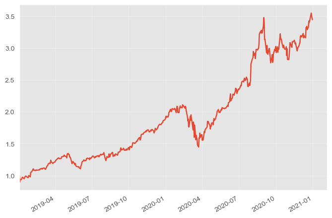
Constructing a price index#
1+aapl['ret'].head()
date
2019-01-02    1.001141
2019-01-03    0.900393
2019-01-04    1.042689
2019-01-07    0.997774
2019-01-08    1.019063
Name: ret, dtype: float64
ax = (1+aapl['ret']).cumprod().plot(xlabel='')
ax.grid(alpha=0.3)
ax.set_xlim(aapl.index[0], None)
plt.show()
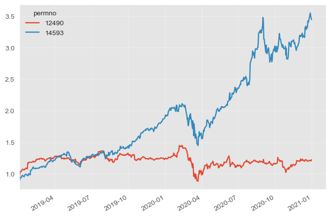
rets = db.raw_sql("""
                  SELECT permno, dlycaldt, dlyret
                  FROM crsp.dsf_v2
                  WHERE permno IN (14593, 12490)
                  AND dlycaldt >= '01/01/2019' AND dlycaldt <= '12/31/2020'
                  """, date_cols=['dlycaldt'])
rets.head()
| permno | dlycaldt | dlyret | |
|---|---|---|---|
| 0 | 12490 | 2019-01-02 | 0.013548 |
| 1 | 12490 | 2019-01-03 | -0.019964 |
| 2 | 12490 | 2019-01-04 | 0.039058 |
| 3 | 12490 | 2019-01-07 | 0.007075 |
| 4 | 12490 | 2019-01-08 | 0.014219 |
rets = rets.pivot(index='dlycaldt', columns='permno', values='dlyret')

rets.head()
| permno | 12490 | 14593 |
|---|---|---|
| dlycaldt | ||
| 2019-01-02 | 0.013548 | 0.001141 |
| 2019-01-03 | -0.019964 | -0.099607 |
| 2019-01-04 | 0.039058 | 0.042689 |
| 2019-01-07 | 0.007075 | -0.002226 |
| 2019-01-08 | 0.014219 | 0.019063 |
ax = (1+rets).cumprod().plot(xlabel='')
ax.grid(alpha=0.3)
ax.set_xlim(rets.index[0], None)
plt.show()
Exercise
Calculate the total return for Apple during the period of April–June, 2020 three different ways:
Use the price index we just created to calculate the desired return.
Aggregate the daily return series.
Separately download the monthly returns from CRSP and aggregate those.
Verify that all three methods yield the same result.
Solution
# using a price index
pidx = (1+rets[14593]).cumprod()
r1 = pidx.loc['2020-06-30'] / pidx.loc['2020-03-31'] - 1

# aggregating daily returns
r2 = rets[14593].resample('QE').apply(lambda x: (1+x).prod()-1).loc['2020-06']

# using monthly returns
mthrets = db.raw_sql("""
                     SELECT mthcaldt, mthret
                     FROM crsp.msf_v2
                     WHERE permno = 14593 and mthcaldt between '4/1/2020' and '6/30/2020'
                     """, date_cols=['mthcaldt'], index_col='mthcaldt')

r3 = (1+mthrets).prod() - 1

# check that r1, r2, and r3 are the same
print([x.item() for x in [r1, r2, r3]])
Day and night returns#
Exercise
The SPDR S&P 500 Trust ETF, introduced in 1993, is an exchange-traded fund that tracks the performance of the S&P 500 Index.
Download the complete history of price data for this ETF. You’ll need to first find its
permno.Calculate the return earned while the market is open (Open-to-Close) and the overnight return (Close-to-Open).
Confirm that the total day-time and overnight return equals close-to-close return.
Calculate the volatility of each return. Interpret your finding.
Calculate and plot the cumulative return of the day and night returns. What do you learn from the graph?
Calculate the day and night returns for each year. Create a bar chart showing the returns by year. Do you notice any interesting pattern to the data?
You can read more about this empirical fact in this article in the New York Times. Two recent research articles that further explore this phenomenon are: