
import numpy as np
import pandas as pd

import matplotlib.pyplot as plt

from statsmodels.tsa.ar_model import AutoReg, ar_select_order
from statsmodels.tsa.regime_switching.markov_autoregression import MarkovAutoregression

import pandas_datareader as pdr
Markov Switching model#
A times series \({x_t}\) follows a Markov switching autoregressive model if
with \(\varepsilon_{k,t}\sim N(0,\sigma_k^2)\).
This model has two states or regimes, denoted by \(S_t\), indicating which state we are in at each time. In each state, a different equation describes how \(x_t\) changes over time.
Note
Pay attention to the subscripts; they provide important information. This is saying that the variance, \(\sigma_k^2\), is different for each \(k\) — meaning for each equation, or state of the world, there are two different variances.
The state variable \(S_t\) is a Markov chain with transition probabilities
In words, this says that the probability of transitioning from state 0 to state 1 is \(\eta_0\), and the probability of transitioning from state 1 to state 0 is \(\eta_1\). These \(\eta\)s are additional parameters that we must estimate from the data. Note also that the rows of the transition matrix sum to one.
More generally, we can have a model with \(k\) different states, in which case we have \(k\) equations for \(x_t\) and a \(k\times k\) transition matrix.
GDP growth#
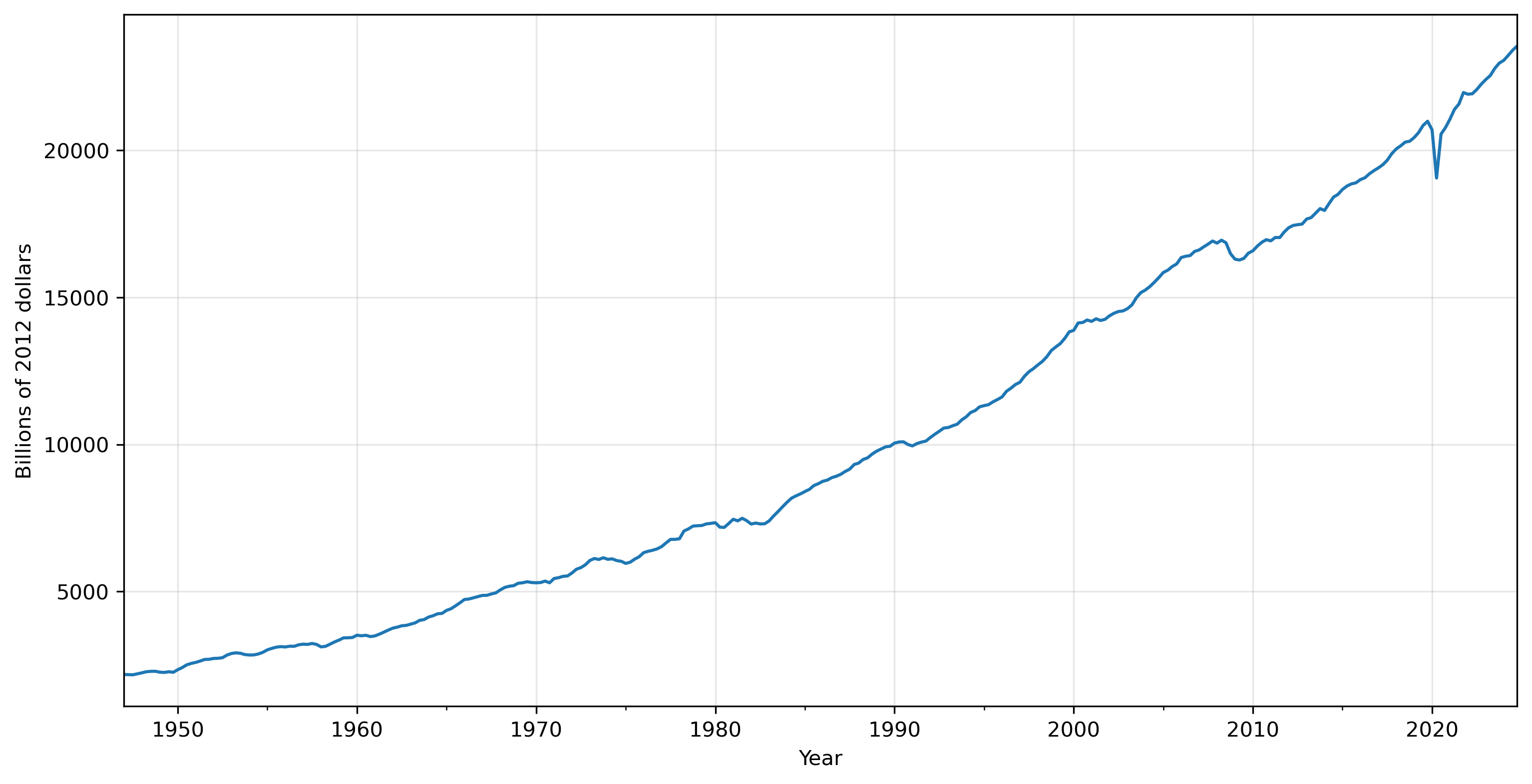
We’ll use the Real Gross Domestic Product series (in Billions of Chained 2012 Dollars, Seasonally Adjusted)
https://fred.stlouisfed.org/series/GDPC1
gdp = pdr.get_data_fred('GDPC1', 1947)

# set index frequency to quarterly
gdp = gdp.asfreq('QS')
gdp.plot(xlabel='Year', ylabel='Billions of 2012 dollars', grid=True, legend=False);
gdpgr = np.log(gdp).diff().dropna()
gdpgr.plot(marker='.', title='GDP Growth', legend=None, xlabel='', grid=True);
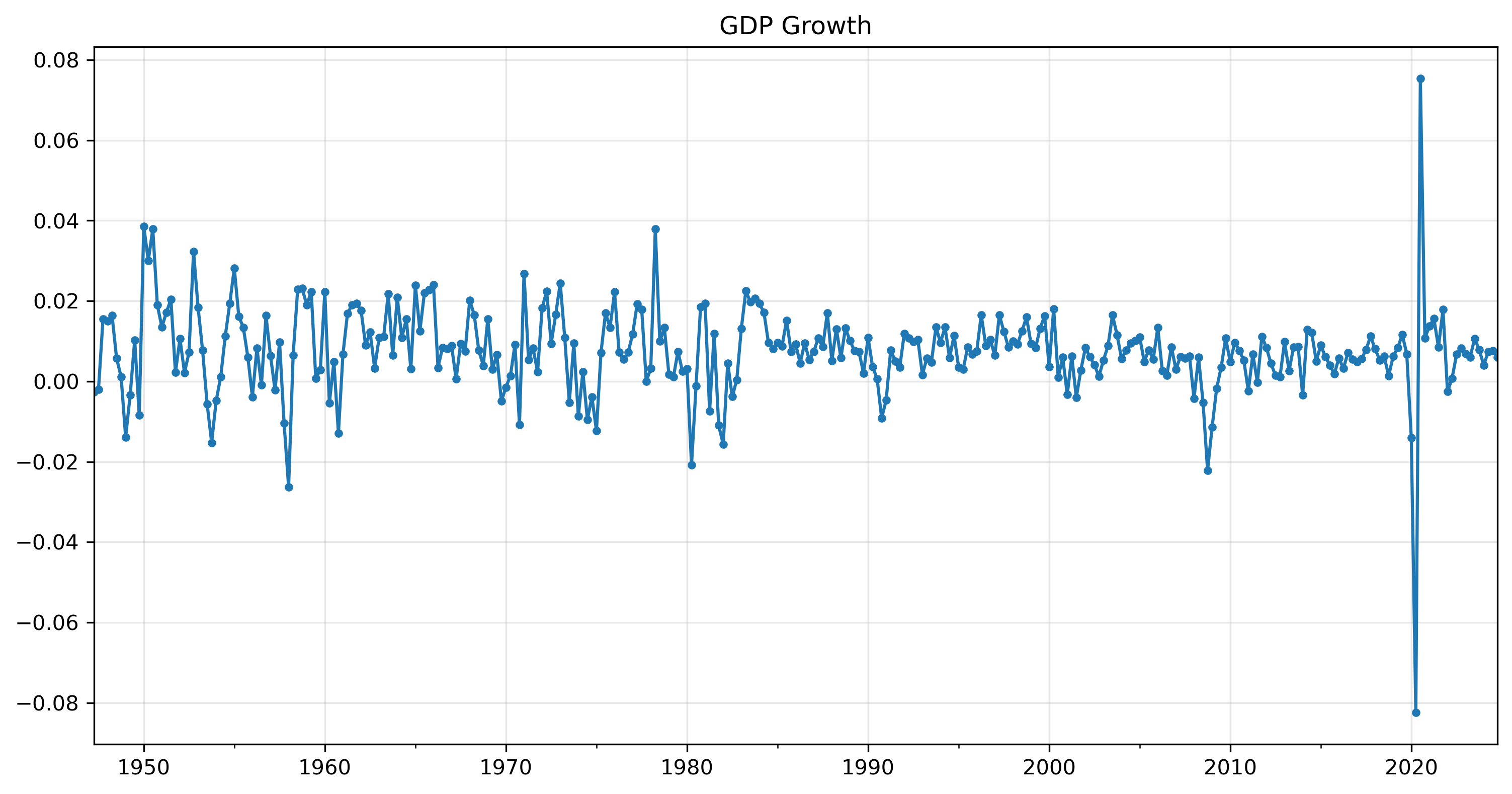
# restrict series to pre-COVID period
gdpgr = gdpgr.loc[:'2019']
gdpgr.describe()
| GDPC1 | |
|---|---|
| count | 291.000000 |
| mean | 0.007778 |
| std | 0.009282 |
| min | -0.026302 |
| 25% | 0.003114 |
| 50% | 0.007701 |
| 75% | 0.012460 |
| max | 0.038564 |
modsel = ar_select_order(gdpgr, maxlag=12, old_names=False, ic='aic')

modsel.ar_lags
[1, 2, 3]
gdpgr_ar3 = AutoReg(gdpgr, 3, old_names=False).fit()
print(gdpgr_ar3.summary())
                            AutoReg Model Results
==============================================================================
Dep. Variable:                  GDPC1   No. Observations:                  291
Model:                     AutoReg(3)   Log Likelihood                 963.626
Method:               Conditional MLE   S.D. of innovations              0.009
Date:                Tue, 15 Apr 2025   AIC                          -1917.253
Time:                        08:01:05   BIC                          -1898.938
Sample:                    01-01-1948   HQIC                         -1909.913
                         - 10-01-2019
==============================================================================
                 coef    std err          z      P>|z|      [0.025      0.975]
------------------------------------------------------------------------------
const          0.0049      0.001      6.467      0.000       0.003       0.006
GDPC1.L1       0.3323      0.058      5.697      0.000       0.218       0.447
GDPC1.L2       0.1519      0.061      2.498      0.012       0.033       0.271
GDPC1.L3      -0.1168      0.058     -2.008      0.045      -0.231      -0.003
                                    Roots
=============================================================================
                  Real          Imaginary           Modulus         Frequency
-----------------------------------------------------------------------------
AR.1           -2.0707           -0.0000j            2.0707           -0.5000
AR.2            1.6856           -1.1375j            2.0335           -0.0945
AR.3            1.6856           +1.1375j            2.0335            0.0945
-----------------------------------------------------------------------------
Start with a simple model where only the mean varies between the states.
gdpgr_mod = MarkovAutoregression(gdpgr, k_regimes=2, order=3, switching_ar=False)

gdpgr_res = gdpgr_mod.fit(disp=True)
print(gdpgr_res.summary())
Optimization terminated successfully.
         Current function value: -3.372021
         Iterations: 57
         Function evaluations: 72
         Gradient evaluations: 72
                         Markov Switching Model Results
================================================================================
Dep. Variable:                    GDPC1   No. Observations:                  288
Model:             MarkovAutoregression   Log Likelihood                 971.142
Date:                  Tue, 15 Apr 2025   AIC                          -1926.284
Time:                          08:01:07   BIC                          -1896.980
Sample:                      04-01-1947   HQIC                         -1914.541
                           - 10-01-2019
Covariance Type:                 approx
                             Regime 0 parameters
==============================================================================
                 coef    std err          z      P>|z|      [0.025      0.975]
------------------------------------------------------------------------------
const         -0.0136      0.004     -3.591      0.000      -0.021      -0.006
                             Regime 1 parameters
==============================================================================
                 coef    std err          z      P>|z|      [0.025      0.975]
------------------------------------------------------------------------------
const          0.0084      0.001     11.122      0.000       0.007       0.010
                           Non-switching parameters
==============================================================================
                 coef    std err          z      P>|z|      [0.025      0.975]
------------------------------------------------------------------------------
sigma2      5.673e-05   5.48e-06     10.347      0.000     4.6e-05    6.75e-05
ar.L1          0.3864      0.061      6.299      0.000       0.266       0.507
ar.L2          0.2276      0.078      2.924      0.003       0.075       0.380
ar.L3         -0.2170      0.070     -3.117      0.002      -0.353      -0.081
                         Regime transition parameters
==============================================================================
                 coef    std err          z      P>|z|      [0.025      0.975]
------------------------------------------------------------------------------
p[0->0]       3.2e-12        nan        nan        nan         nan         nan
p[1->0]        0.0293      0.015      1.961      0.050    1.44e-05       0.059
==============================================================================

Warnings:
[1] Covariance matrix calculated using numerical (complex-step) differentiation.
Looking at the estimates of the transition probability, it’s clear that the optimizer didn’t find a good solution, which is why the standard errors on the probabilities are infinite. The likelihood function was likely not actually maximized. Let’s try again with a bit more control over the optmizer.
We should get a log-likelihood of about 974.
gdpgr_mod2 = MarkovAutoregression(gdpgr, k_regimes=2, order=3, switching_ar=False)
Optimization terminated successfully.
         Current function value: -3.381781
         Iterations: 30
         Function evaluations: 38
         Gradient evaluations: 38
                         Markov Switching Model Results
================================================================================
Dep. Variable:                    GDPC1   No. Observations:                  288
Model:             MarkovAutoregression   Log Likelihood                 973.953
Date:                  Tue, 15 Apr 2025   AIC                          -1931.906
Time:                          08:01:54   BIC                          -1902.602
Sample:                      04-01-1947   HQIC                         -1920.163
                           - 10-01-2019
Covariance Type:                 approx
                             Regime 0 parameters
==============================================================================
                 coef    std err          z      P>|z|      [0.025      0.975]
------------------------------------------------------------------------------
const         -0.0122      0.003     -4.177      0.000      -0.018      -0.006
                             Regime 1 parameters
==============================================================================
                 coef    std err          z      P>|z|      [0.025      0.975]
------------------------------------------------------------------------------
const          0.0089      0.001     11.241      0.000       0.007       0.010
                           Non-switching parameters
==============================================================================
                 coef    std err          z      P>|z|      [0.025      0.975]
------------------------------------------------------------------------------
sigma2      5.015e-05   5.27e-06      9.518      0.000    3.98e-05    6.05e-05
ar.L1          0.4410      0.066      6.717      0.000       0.312       0.570
ar.L2          0.2594      0.069      3.748      0.000       0.124       0.395
ar.L3         -0.2662      0.069     -3.836      0.000      -0.402      -0.130
                         Regime transition parameters
==============================================================================
                 coef    std err          z      P>|z|      [0.025      0.975]
------------------------------------------------------------------------------
p[0->0]        0.2316      0.138      1.682      0.093      -0.038       0.501
p[1->0]        0.0416      0.018      2.319      0.020       0.006       0.077
==============================================================================

Warnings:
[1] Covariance matrix calculated using numerical (complex-step) differentiation.
The DataFrame below shows how the parameter values changed through the iteration steps.
param_store.param_history
| p[0->0] | p[1->0] | const[0] | const[1] | sigma2 | ar.L1 | ar.L2 | ar.L3 | Log-Like | |
|---|---|---|---|---|---|---|---|---|---|
| iteration | |||||||||
| 1 | 0.207039 | 0.028825 | -0.011880 | 0.008544 | 0.000056 | 0.292192 | 0.163504 | -0.163383 | 969.920612 |
| 2 | 0.207039 | 0.028825 | -0.011911 | 0.008622 | 0.000056 | 0.292201 | 0.163514 | -0.163386 | 969.928504 |
| 3 | 0.207039 | 0.028825 | -0.012120 | 0.008609 | 0.000056 | 0.292273 | 0.163591 | -0.163407 | 969.942013 |
| 4 | 0.207046 | 0.028832 | -0.012225 | 0.008616 | 0.000056 | 0.302166 | 0.174178 | -0.166545 | 970.485798 |
| 5 | 0.207056 | 0.028874 | -0.012492 | 0.008636 | 0.000055 | 0.324868 | 0.194296 | -0.183971 | 971.495154 |
| 6 | 0.207088 | 0.029050 | -0.013029 | 0.008694 | 0.000052 | 0.374596 | 0.236686 | -0.227985 | 973.074853 |
| 7 | 0.207216 | 0.029423 | -0.013549 | 0.008761 | 0.000051 | 0.430162 | 0.277880 | -0.274869 | 973.552750 |
| 8 | 0.207285 | 0.029530 | -0.013189 | 0.008739 | 0.000052 | 0.425794 | 0.263744 | -0.262679 | 973.625840 |
| 9 | 0.207402 | 0.029738 | -0.013306 | 0.008743 | 0.000052 | 0.428603 | 0.256207 | -0.258248 | 973.652543 |
| 10 | 0.207699 | 0.030254 | -0.013267 | 0.008752 | 0.000051 | 0.437020 | 0.248603 | -0.255674 | 973.679306 |
| 11 | 0.208042 | 0.030826 | -0.013247 | 0.008758 | 0.000051 | 0.441883 | 0.246273 | -0.256050 | 973.699708 |
| 12 | 0.208680 | 0.031882 | -0.013168 | 0.008769 | 0.000051 | 0.446550 | 0.244904 | -0.257256 | 973.736175 |
| 13 | 0.209896 | 0.033938 | -0.013000 | 0.008788 | 0.000051 | 0.451137 | 0.244816 | -0.259621 | 973.799291 |
| 14 | 0.212335 | 0.038309 | -0.012621 | 0.008827 | 0.000050 | 0.454306 | 0.247976 | -0.264062 | 973.890612 |
| 15 | 0.214269 | 0.041913 | -0.012260 | 0.008860 | 0.000050 | 0.450723 | 0.253989 | -0.267176 | 973.931406 |
| 16 | 0.214585 | 0.042268 | -0.012190 | 0.008867 | 0.000050 | 0.445428 | 0.257661 | -0.267334 | 973.941682 |
| 17 | 0.214557 | 0.041812 | -0.012226 | 0.008863 | 0.000050 | 0.440825 | 0.259826 | -0.266630 | 973.944946 |
| 18 | 0.214592 | 0.041656 | -0.012239 | 0.008859 | 0.000050 | 0.440421 | 0.259797 | -0.266355 | 973.945102 |
| 19 | 0.214790 | 0.041510 | -0.012255 | 0.008855 | 0.000050 | 0.440127 | 0.259697 | -0.266056 | 973.945308 |
| 20 | 0.215271 | 0.041369 | -0.012270 | 0.008851 | 0.000050 | 0.439869 | 0.259581 | -0.265729 | 973.945669 |
| 21 | 0.216236 | 0.041225 | -0.012284 | 0.008846 | 0.000050 | 0.439625 | 0.259454 | -0.265371 | 973.946315 |
| 22 | 0.218119 | 0.041073 | -0.012298 | 0.008842 | 0.000050 | 0.439407 | 0.259305 | -0.264968 | 973.947459 |
| 23 | 0.221823 | 0.040935 | -0.012307 | 0.008839 | 0.000050 | 0.439297 | 0.259134 | -0.264572 | 973.949340 |
| 24 | 0.229164 | 0.040937 | -0.012293 | 0.008842 | 0.000050 | 0.439619 | 0.258998 | -0.264486 | 973.951655 |
| 25 | 0.231531 | 0.041167 | -0.012263 | 0.008851 | 0.000050 | 0.440169 | 0.259116 | -0.265053 | 973.952458 |
| 26 | 0.232263 | 0.041530 | -0.012220 | 0.008864 | 0.000050 | 0.440909 | 0.259364 | -0.266000 | 973.952934 |
| 27 | 0.231739 | 0.041597 | -0.012213 | 0.008866 | 0.000050 | 0.441025 | 0.259427 | -0.266200 | 973.952960 |
| 28 | 0.231586 | 0.041600 | -0.012213 | 0.008866 | 0.000050 | 0.441026 | 0.259434 | -0.266218 | 973.952960 |
| 29 | 0.231578 | 0.041599 | -0.012213 | 0.008866 | 0.000050 | 0.441024 | 0.259433 | -0.266219 | 973.952961 |
| 30 | 0.231578 | 0.041599 | -0.012213 | 0.008866 | 0.000050 | 0.441024 | 0.259433 | -0.266220 | 973.952961 |
We have two states, with constant terms \(\phi_{0,0} = -0.0122\) and \(\phi_{0,1} = 0.0089\). Clearly, the first state is a low-growth (or “recession”) state and the second state is the high-growth state.
The transition probability matrix is
so if you’re in the high-growth state, there’s about a 96% chance you’ll stay there, but if you’re in the recession state there’s a 77% chance you’ll transition out of it. If you think about how long recessions last, this makes perfect sense.
The expected duration of the two states are given by \(\frac{1}{0.7685}\) and \(\frac{1}{0.0415}.\)
gdpgr_res2.expected_durations
array([ 1.30136812, 24.0389007 ])
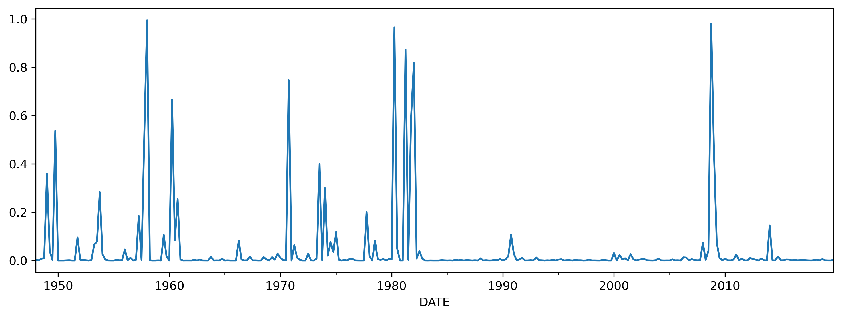
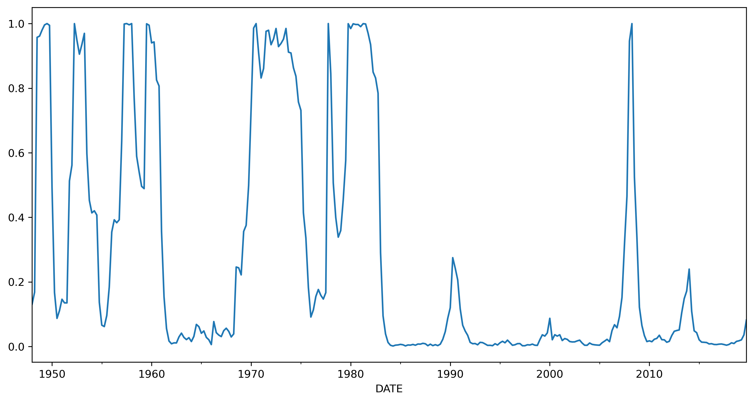
Let’s look at the filtered probabilities of state 0.
gdpgr_res2.filtered_marginal_probabilities[0].plot(figsize=(12,4))
<Axes: xlabel='DATE'>
# get NBER recessions data
usrec = pdr.get_data_fred('USREC', start=1947).squeeze()
The Great Moderation#
ax = gdpgr.loc[:'2019'].plot(figsize=(16,6), marker='.')

gdpgr.rolling(4*3).std().plot(ax=ax)

ax.legend(['GDP', 'Std.Dev.'])
<matplotlib.legend.Legend at 0x176d657f0>
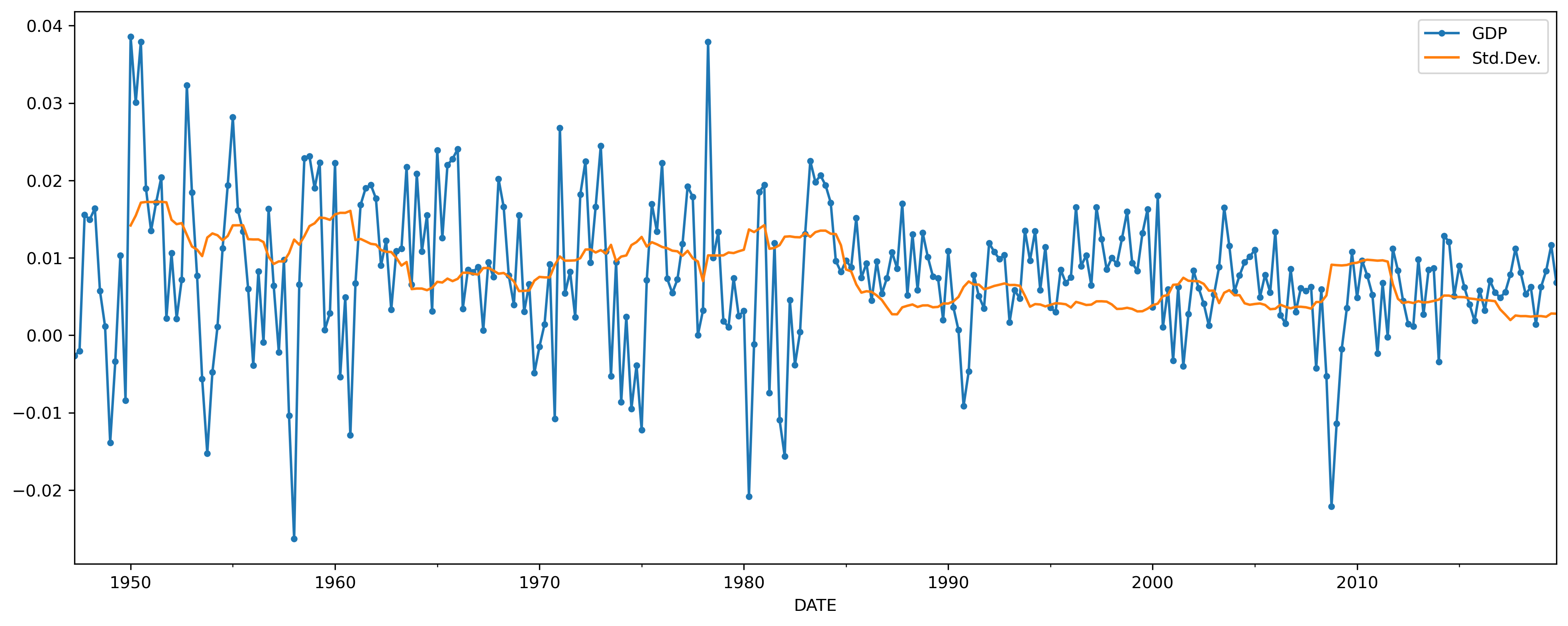
The volatility in the series after 1985 is about half of what it is before that.
gdpgr[:'1985'].std()
GDPC1    0.011468
dtype: float64
gdpgr['1985':].std()
GDPC1    0.005629
dtype: float64
This decline in the volatility of GDP growth is known as the Great Moderation.
We can estimate a Markov Switching Model where the autoregressive structure changes depending on which state we are in.
mod_gdpgr2 = MarkovAutoregression(gdpgr, k_regimes=2, order=3,
                                  switching_ar=True,
                                  switching_variance=True)
res_gdpgr2 = mod_gdpgr2.fit(disp=True)
print(res_gdpgr2.summary())
Optimization terminated successfully.
         Current function value: -3.464792
         Iterations: 60
         Function evaluations: 74
         Gradient evaluations: 74
                         Markov Switching Model Results
================================================================================
Dep. Variable:                    GDPC1   No. Observations:                  288
Model:             MarkovAutoregression   Log Likelihood                 997.860
Date:                  Tue, 15 Apr 2025   AIC                          -1971.720
Time:                          08:03:14   BIC                          -1927.765
Sample:                      04-01-1947   HQIC                         -1954.106
                           - 10-01-2019
Covariance Type:                 approx
                             Regime 0 parameters
==============================================================================
                 coef    std err          z      P>|z|      [0.025      0.975]
------------------------------------------------------------------------------
const          0.0039      0.003      1.461      0.144      -0.001       0.009
sigma2         0.0002   4.68e-05      3.710      0.000    8.19e-05       0.000
ar.L1          0.1701      0.294      0.578      0.563      -0.406       0.747
ar.L2          0.0333      0.152      0.220      0.826      -0.264       0.330
ar.L3         -0.0172      0.197     -0.088      0.930      -0.403       0.369
                             Regime 1 parameters
==============================================================================
                 coef    std err          z      P>|z|      [0.025      0.975]
------------------------------------------------------------------------------
const          0.0089      0.001      9.467      0.000       0.007       0.011
sigma2      2.747e-05   3.59e-06      7.645      0.000    2.04e-05    3.45e-05
ar.L1          0.3493      0.095      3.680      0.000       0.163       0.535
ar.L2          0.3082      0.076      4.041      0.000       0.159       0.458
ar.L3         -0.2095      0.086     -2.438      0.015      -0.378      -0.041
                         Regime transition parameters
==============================================================================
                 coef    std err          z      P>|z|      [0.025      0.975]
------------------------------------------------------------------------------
p[0->0]        0.8760      0.131      6.674      0.000       0.619       1.133
p[1->0]        0.0464      0.029      1.605      0.108      -0.010       0.103
==============================================================================

Warnings:
[1] Covariance matrix calculated using numerical (complex-step) differentiation.
The main difference in the models is the huge difference in the estimate of the volatility parameters in each regime:
res_gdpgr2.params.loc['sigma2[0]'] / res_gdpgr2.params.loc['sigma2[1]']
np.float64(6.318021262238154)
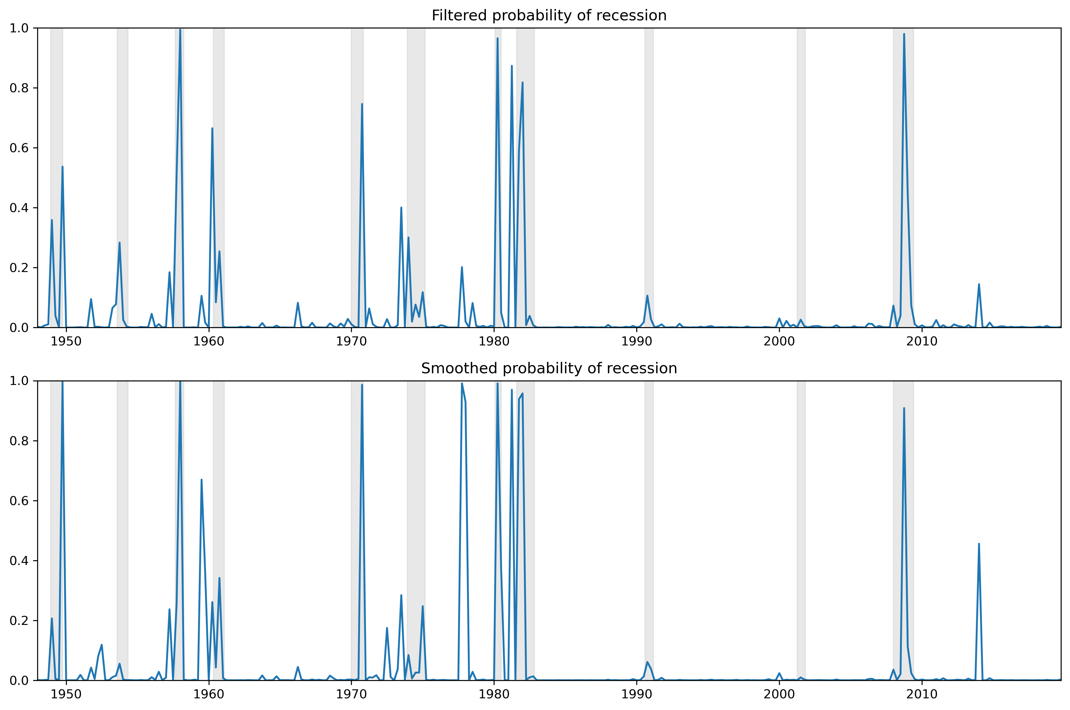
res_gdpgr2.smoothed_marginal_probabilities[0].plot();
import statsmodels.api as sm

from statsmodels.tsa import stattools as st
fig, (ax1, ax2) = plt.subplots(2,1, figsize=(16,8))
plt.subplots_adjust(hspace=0.25)

res_gdpgr2.resid.plot(ax=ax1)

fig = sm.graphics.tsa.plot_acf(res_gdpgr2.resid.values, lags=12, ax=ax2)
ax2.set_title('Residuals')
ax2.set_ylabel('ACF')

plt.show()
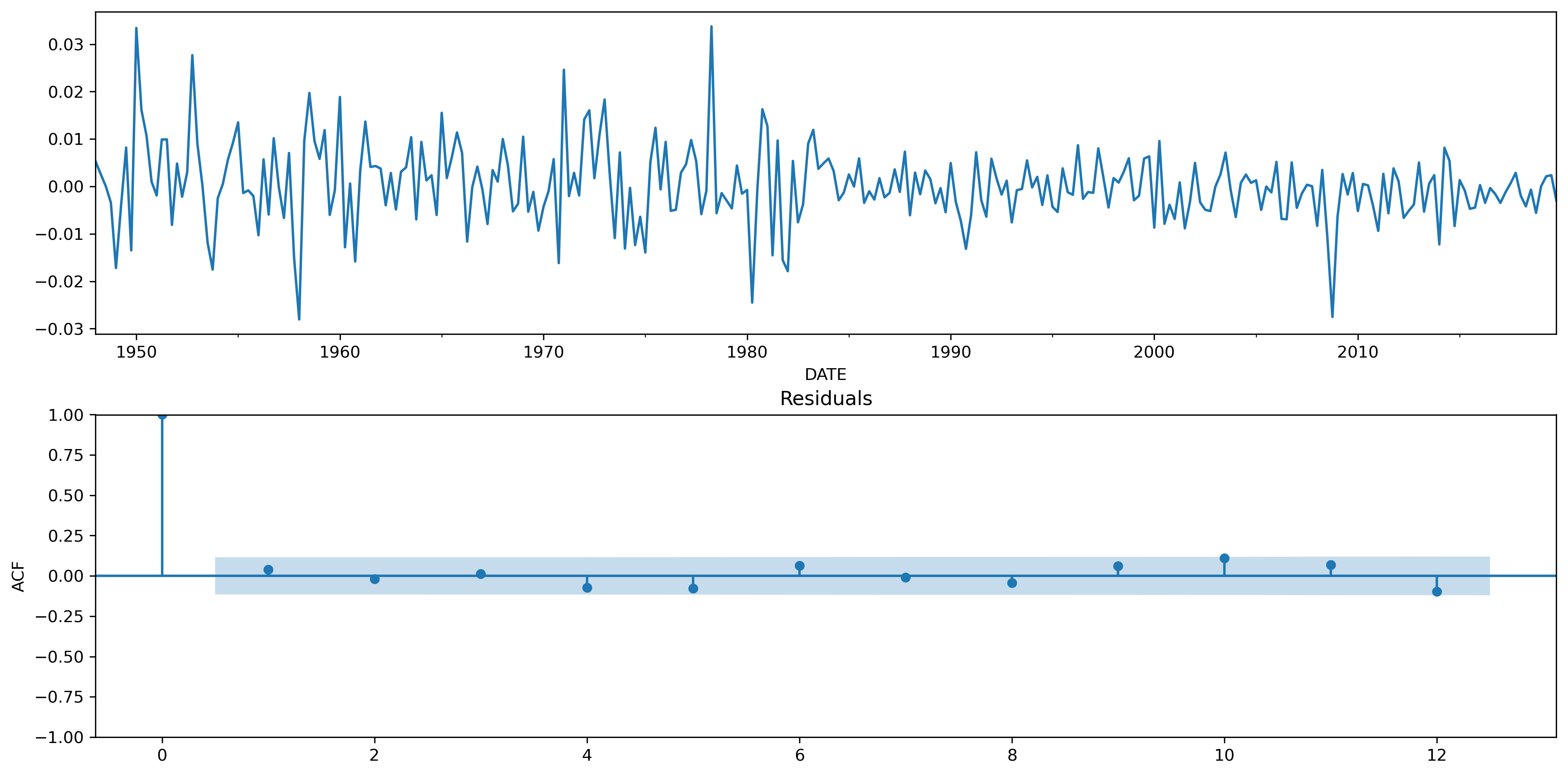
acf, qstats, pvals = st.acf(res_gdpgr2.resid, nlags=12, qstat=True)
pvals
array([0.49704508, 0.75425769, 0.8932877 , 0.70526199, 0.56530032,
       0.52849255, 0.64202275, 0.68052737, 0.65837221, 0.40848839,
       0.37669856, 0.26197076])