
Shiller’s CAPE#
Bob Shiller is a professor of economics at Yale and winner of the 2013 Nobel Prize in economics for his empirical analysis of asset prices.
Shiller developed the Cyclically Adjusted Price-to-Earnings (CAPE) Ratio as a valuation metric for stock markets. CAPE is measured as the ratio of the current price of a market index (e.g. the S&P 500) to the average real earnings over the past ten years for stocks in the index.
Let’s calculate CAPE using data from Shiller’s website.
The URL for current file is:
https://img1.wsimg.com/blobby/go/e5e77e0b-59d1-44d9-ab25-4763ac982e53/downloads/25d6827d-c04b-447a-bb6d-918d5d88be49/ie_data.xls?ver=1770307872442.
I have saved this URL in a variable called file_loc.
shiller = pd.read_excel(file_loc,
                        sheet_name='Data', skiprows=range(7),
                        skipfooter=1, usecols='A:E',
                        dtype={'Date':str})
shiller
| Date | P | D | E | CPI | |
|---|---|---|---|---|---|
| 0 | 1871.01 | 4.440000 | 0.26000 | 0.4 | 12.464061 |
| 1 | 1871.02 | 4.500000 | 0.26000 | 0.4 | 12.844641 |
| 2 | 1871.03 | 4.610000 | 0.26000 | 0.4 | 13.034972 |
| 3 | 1871.04 | 4.740000 | 0.26000 | 0.4 | 12.559226 |
| 4 | 1871.05 | 4.860000 | 0.26000 | 0.4 | 12.273812 |
| ... | ... | ... | ... | ... | ... |
| 1857 | 2025.1 | 6735.691739 | 78.62672 | NaN | 325.212000 |
| 1858 | 2025.11 | 6740.885789 | 78.77344 | NaN | 324.122000 |
| 1859 | 2025.12 | 6853.025455 | 78.92016 | NaN | 324.054000 |
| 1860 | 2026.01 | 6929.122000 | NaN | NaN | 324.020000 |
| 1861 | 2026.02 | 6882.720000 | NaN | NaN | 324.003000 |
1862 rows × 5 columns
We’ll use the Date column to add a ‘DatetimeIndex’.
shiller['Date'] = pd.date_range(start='1871-01-31', periods=len(shiller), freq='ME')

shiller = shiller.set_index('Date')
shiller.info()
<class 'pandas.core.frame.DataFrame'>
DatetimeIndex: 1862 entries, 1871-01-31 to 2026-02-28
Data columns (total 4 columns):
 #   Column  Non-Null Count  Dtype
---  ------  --------------  -----
 0   P       1862 non-null   float64
 1   D       1860 non-null   float64
 2   E       1857 non-null   float64
 3   CPI     1862 non-null   float64
dtypes: float64(4)
memory usage: 72.7 KB
shiller
| P | D | E | CPI | |
|---|---|---|---|---|
| Date | ||||
| 1871-01-31 | 4.440000 | 0.26000 | 0.4 | 12.464061 |
| 1871-02-28 | 4.500000 | 0.26000 | 0.4 | 12.844641 |
| 1871-03-31 | 4.610000 | 0.26000 | 0.4 | 13.034972 |
| 1871-04-30 | 4.740000 | 0.26000 | 0.4 | 12.559226 |
| 1871-05-31 | 4.860000 | 0.26000 | 0.4 | 12.273812 |
| ... | ... | ... | ... | ... |
| 2025-10-31 | 6735.691739 | 78.62672 | NaN | 325.212000 |
| 2025-11-30 | 6740.885789 | 78.77344 | NaN | 324.122000 |
| 2025-12-31 | 6853.025455 | 78.92016 | NaN | 324.054000 |
| 2026-01-31 | 6929.122000 | NaN | NaN | 324.020000 |
| 2026-02-28 | 6882.720000 | NaN | NaN | 324.003000 |
1862 rows × 4 columns
To convert all the data to “real” terms, we need to adjust for inflation. We do this by calculating how much the CPI has changed from each year until the last year in the sample. (Shiller uses the non-seasonally adjusted CPI data, which starts in 1913, along with another price series that goes earlier.)
Exercise
Use the data to calculate the total inflation rate during 2020–2025.
Solution
shiller['CPI'].loc['2025-12-31'] / shiller['CPI'].loc['2019-12-31'] - 1
Total inflation was 26.1% during this period.
We’ll create a CPI factor using the number from a few months before the end of the series because the most recent values are estimates.
shiller['CPI_factor'] = shiller['CPI'] / shiller['CPI'].iloc[-3]
shiller.head()
| P | D | E | CPI | CPI_factor | |
|---|---|---|---|---|---|
| Date | |||||
| 1871-01-31 | 4.44 | 0.26 | 0.4 | 12.464061 | 0.038463 |
| 1871-02-28 | 4.50 | 0.26 | 0.4 | 12.844641 | 0.039637 |
| 1871-03-31 | 4.61 | 0.26 | 0.4 | 13.034972 | 0.040225 |
| 1871-04-30 | 4.74 | 0.26 | 0.4 | 12.559226 | 0.038757 |
| 1871-05-31 | 4.86 | 0.26 | 0.4 | 12.273812 | 0.037876 |
shiller.tail(12)
| P | D | E | CPI | CPI_factor | |
|---|---|---|---|---|---|
| Date | |||||
| 2025-03-31 | 5683.983333 | 76.145301 | 216.690000 | 319.799 | 0.986869 |
| 2025-04-30 | 5369.495714 | 76.546867 | 218.636667 | 320.795 | 0.989943 |
| 2025-05-31 | 5810.919524 | 76.948434 | 220.583333 | 321.465 | 0.992011 |
| 2025-06-30 | 6029.951500 | 77.350000 | 222.530000 | 322.561 | 0.995393 |
| 2025-07-31 | 6296.498182 | 77.726667 | 226.770000 | 323.048 | 0.996896 |
| 2025-08-31 | 6408.949524 | 78.103333 | 231.010000 | 323.976 | 0.999759 |
| 2025-09-30 | 6584.018095 | 78.480000 | 235.250000 | 324.800 | 1.002302 |
| 2025-10-31 | 6735.691739 | 78.626720 | NaN | 325.212 | 1.003573 |
| 2025-11-30 | 6740.885789 | 78.773440 | NaN | 324.122 | 1.000210 |
| 2025-12-31 | 6853.025455 | 78.920160 | NaN | 324.054 | 1.000000 |
| 2026-01-31 | 6929.122000 | NaN | NaN | 324.020 | 0.999895 |
| 2026-02-28 | 6882.720000 | NaN | NaN | 324.003 | 0.999843 |
shiller['p_real'] = shiller['P'] / shiller['CPI_factor']
shiller['d_real'] = shiller['D'] / shiller['CPI_factor']
shiller['e_real'] = shiller['E'] / shiller['CPI_factor']
shiller = shiller.reindex(columns=['p_real', 'd_real', 'e_real'])
shiller.head()
| p_real | d_real | e_real | |
|---|---|---|---|
| Date | |||
| 1871-01-31 | 115.435871 | 6.759758 | 10.399628 |
| 1871-02-28 | 113.529289 | 6.559470 | 10.091492 |
| 1871-03-31 | 114.606226 | 6.463692 | 9.944141 |
| 1871-04-30 | 122.301797 | 6.708537 | 10.320827 |
| 1871-05-31 | 128.314047 | 6.864538 | 10.560827 |
shiller.tail(15)
| p_real | d_real | e_real | |
|---|---|---|---|
| Date | |||
| 2024-12-31 | 6171.825434 | 76.835574 | 215.796420 |
| 2025-01-31 | 6099.662594 | 76.782344 | 216.609972 |
| 2025-02-28 | 6132.786084 | 76.887310 | 217.859309 |
| 2025-03-31 | 5759.610052 | 77.158432 | 219.573111 |
| 2025-04-30 | 5424.045151 | 77.324517 | 220.857826 |
| 2025-05-31 | 5857.719240 | 77.568157 | 222.359857 |
| 2025-06-30 | 6057.861624 | 77.708021 | 223.559998 |
| 2025-07-31 | 6316.106033 | 77.968714 | 227.476182 |
| 2025-08-31 | 6410.492533 | 78.122137 | 231.065618 |
| 2025-09-30 | 6568.895935 | 78.299747 | 234.709678 |
| 2025-10-31 | 6711.707596 | 78.346750 | NaN |
| 2025-11-30 | 6739.471568 | 78.756914 | NaN |
| 2025-12-31 | 6853.025455 | 78.920160 | NaN |
| 2026-01-31 | 6929.849085 | NaN | NaN |
| 2026-02-28 | 6883.803381 | NaN | NaN |
Next we’ll calculate a rolling 10-year average of earnings.
earn_ma = shiller['e_real'].rolling(window=120, min_periods=100).mean()

earn_ma.iloc[95:105]
Date
1878-12-31          NaN
1879-01-31          NaN
1879-02-28          NaN
1879-03-31          NaN
1879-04-30    10.955256
1879-05-31    10.979792
1879-06-30    11.007675
1879-07-31    11.035686
1879-08-31    11.065405
1879-09-30    11.092137
Name: e_real, dtype: float64
The value of CAPE is the current price value divided by the rolling average lagged one period. We do this by calling .shift to shift the time series one period.
shiller['CAPE'] = shiller['p_real'] / earn_ma.shift()

shiller.tail(12)
| p_real | d_real | e_real | CAPE | |
|---|---|---|---|---|
| Date | ||||
| 2025-03-31 | 5759.610052 | 77.158432 | 219.573111 | 34.784750 |
| 2025-04-30 | 5424.045151 | 77.324517 | 220.857826 | 32.621270 |
| 2025-05-31 | 5857.719240 | 77.568157 | 222.359857 | 35.076697 |
| 2025-06-30 | 6057.861624 | 77.708021 | 223.559998 | 36.111092 |
| 2025-07-31 | 6316.106033 | 77.968714 | 227.476182 | 37.474246 |
| 2025-08-31 | 6410.492533 | 78.122137 | 231.065618 | 37.846145 |
| 2025-09-30 | 6568.895935 | 78.299747 | 234.709678 | 38.580387 |
| 2025-10-31 | 6711.707596 | 78.346750 | NaN | 39.205692 |
| 2025-11-30 | 6739.471568 | 78.756914 | NaN | 39.272363 |
| 2025-12-31 | 6853.025455 | 78.920160 | NaN | 39.832601 |
| 2026-01-31 | 6929.849085 | NaN | NaN | 40.172372 |
| 2026-02-28 | 6883.803381 | NaN | NaN | 39.797673 |
Check your understanding
Check your understanding. Why is CAPE not missing at the end of the series?
Next, we’ll add a recession indicator variable (1 or 0) by accessing data from the St. Louis Federal Reserve data service, FRED using the pandas_datareader.
The particular series we want is at https://fred.stlouisfed.org/series/USREC.
import pandas_datareader as pdr
nber = pdr.get_data_fred('USREC', '1870')
nber.head()
| USREC | |
|---|---|
| DATE | |
| 1870-01-01 | 1 |
| 1870-02-01 | 1 |
| 1870-03-01 | 1 |
| 1870-04-01 | 1 |
| 1870-05-01 | 1 |
nber.mean()
USREC    0.274426
dtype: float64
The easiest way to merge these two dataframes is to adjust the NBER data’s index so that its dates are at the end of the month, like they are in the Shiller data. We do this using the pandas MonthEnd offset function. Since we want to adjust the date to be the end of the current month, we add zero months.
from pandas.tseries.offsets import MonthEnd

nber.index = nber.index + MonthEnd(0)
shiller = shiller.join(nber).dropna()

shiller.head()
| p_real | d_real | e_real | CAPE | USREC | |
|---|---|---|---|---|---|
| Date | |||||
| 1879-05-31 | 156.036733 | 7.457289 | 13.433416 | 14.243094 | 0.0 |
| 1879-06-30 | 158.673595 | 7.613127 | 13.823836 | 14.451421 | 0.0 |
| 1879-07-31 | 159.997056 | 7.591940 | 13.892814 | 14.535046 | 0.0 |
| 1879-08-31 | 161.185153 | 7.655305 | 14.126473 | 14.605812 | 0.0 |
| 1879-09-30 | 161.492602 | 7.462336 | 13.872291 | 14.594369 | 0.0 |
Check your understanding
Why does this joined data series start in May of 1879?
Plotting#
Now we can plot the series and add some other bells and whistles.
import matplotlib.pyplot as plt
from matplotlib.dates import YearLocator
# main plot
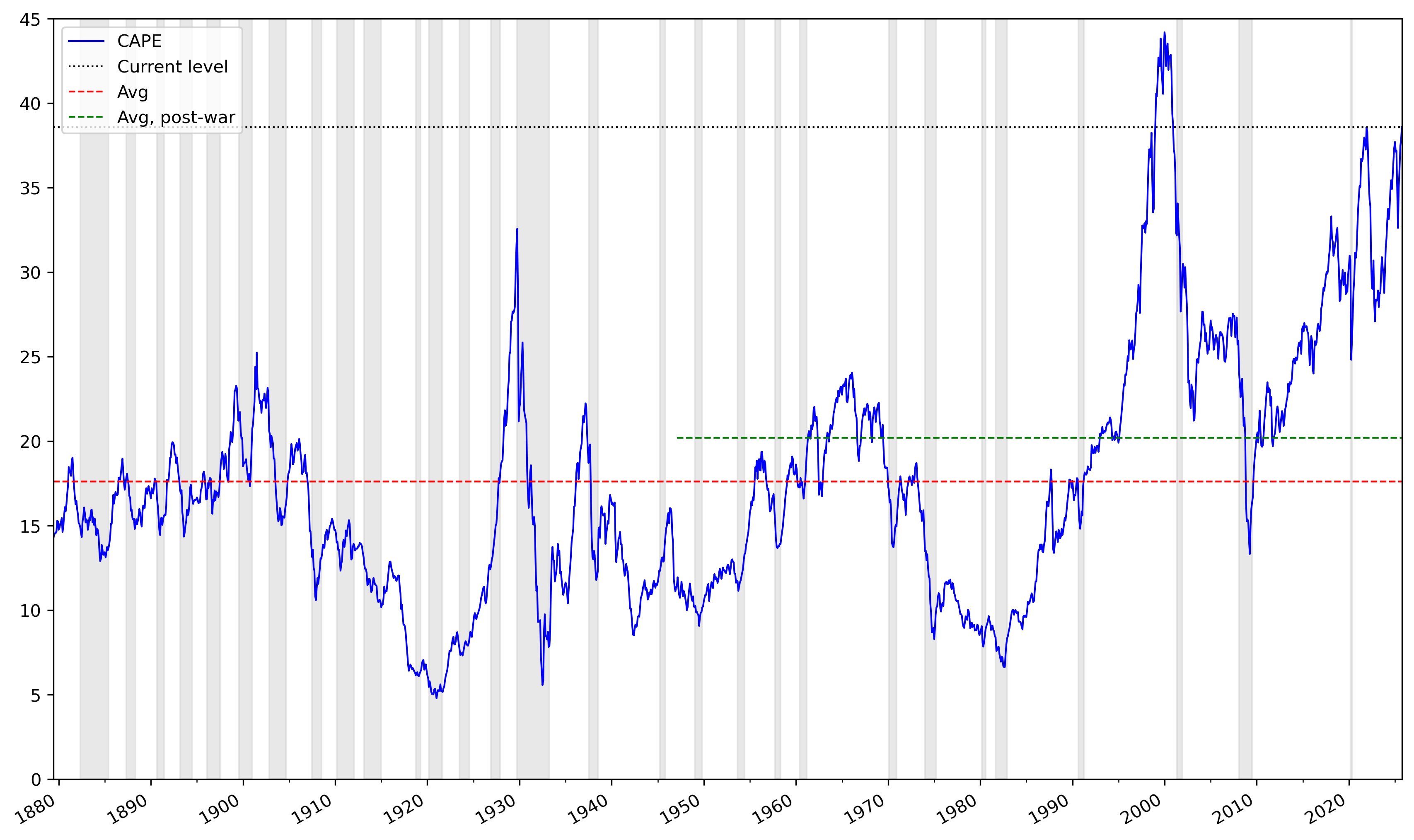
ax = shiller['CAPE'].plot(figsize=(14,9), ylim=(0,45), legend=True, x_compat=True, c='b', lw=1)
# create Series with means and current value repeated
avg = pd.Series(shiller['CAPE'].mean(), index=shiller.index)
avg47 = pd.Series(shiller.loc['1947':,'CAPE'].mean(), index=shiller.loc['1947':].index)
curentval = pd.Series(shiller['CAPE'].iloc[-1], index=shiller.index)
# add lines for means and current value
curentval.plot(ax=ax, label='Current level', legend=True, c='k', ls=':', lw=1)
avg.plot(ax=ax, label='Avg', legend=True, c='r', ls='--', lw=1)
avg47.plot(ax=ax, label='Avg, post-war', legend=True, c='g', ls='--', lw=1)
plt.legend(loc='upper left', fontsize='medium')
# add shaded areas for recessions
ax.fill_between(shiller['CAPE'].index, 0, 45, where=shiller['USREC']==1,
facecolor='lightgrey', edgecolor='lightgrey', alpha=0.5)
# change year locations
yrs10 = YearLocator(10)
yrs5 = YearLocator(5)
ax.xaxis.set_major_locator(yrs10)
ax.xaxis.set_minor_locator(yrs5)
ax.set_xlim(left=shiller.index[0], right=shiller.index[-1])
ax.set_xlabel('')
plt.show()
Correlations#
Let’s calculate future 2- and 5-year returns. We do this by dividing the price in 2 or 5 years by the price “today”.
The forward returns is
Note that we cannot calculate this using pct_change.
shiller['ret2yr'] = shiller['p_real'].shift(-2*12) / shiller['p_real'] - 1
shiller['ret5yr'] = shiller['p_real'].shift(-5*12) / shiller['p_real'] - 1
shiller.dropna()
| p_real | d_real | e_real | CAPE | USREC | ret2yr | ret5yr | |
|---|---|---|---|---|---|---|---|
| Date | |||||||
| 1879-05-31 | 156.036733 | 7.457289 | 13.433416 | 14.243094 | 0.0 | 0.418777 | 0.091373 |
| 1879-06-30 | 158.673595 | 7.613127 | 13.823836 | 14.451421 | 0.0 | 0.412371 | 0.029384 |
| 1879-07-31 | 159.997056 | 7.591940 | 13.892814 | 14.535046 | 0.0 | 0.338353 | 0.031959 |
| 1879-08-31 | 161.185153 | 7.655305 | 14.126473 | 14.605812 | 0.0 | 0.271915 | 0.088661 |
| 1879-09-30 | 161.492602 | 7.462336 | 13.872291 | 14.594369 | 0.0 | 0.231891 | 0.063768 |
| ... | ... | ... | ... | ... | ... | ... | ... |
| 2020-05-31 | 3690.074336 | 75.387123 | 132.620054 | 27.328481 | 0.0 | 0.213890 | 0.587426 |
| 2020-06-30 | 3902.596951 | 75.018494 | 124.733331 | 28.838316 | 0.0 | 0.092605 | 0.552264 |
| 2020-07-31 | 4011.724373 | 74.294919 | 123.684510 | 29.599195 | 0.0 | 0.066495 | 0.574412 |
| 2020-08-31 | 4228.630539 | 73.716452 | 122.875992 | 31.158209 | 0.0 | 0.076015 | 0.515974 |
| 2020-09-30 | 4190.138074 | 73.269471 | 122.285938 | 30.839426 | 0.0 | 0.003305 | 0.567704 |
1697 rows × 7 columns
shiller[['CAPE', 'ret2yr', 'ret5yr']].corr()
| CAPE | ret2yr | ret5yr | |
|---|---|---|---|
| CAPE | 1.000000 | -0.154628 | -0.214495 |
| ret2yr | -0.154628 | 1.000000 | 0.581104 |
| ret5yr | -0.214495 | 0.581104 | 1.000000 |
shiller.loc['1980':, ['CAPE', 'ret2yr', 'ret5yr']].corr()
| CAPE | ret2yr | ret5yr | |
|---|---|---|---|
| CAPE | 1.000000 | -0.270159 | -0.463946 |
| ret2yr | -0.270159 | 1.000000 | 0.590445 |
| ret5yr | -0.463946 | 0.590445 | 1.000000 |
Discussion questions#
How would you interpret these correlation results?
How confident are you that we should believe these correlations? Should you use this result to make investment decisions?
How might changing macroeconomic trends affect the relevance of the CAPE ratio?