
Pseudorandom number generation#
Before continuing our discussion of theoretical aspects of probablity and statistics, it will be useful to have a basic understanding of how computers generate numbers that appear random. These random numbers are used as the basis for Monte Carlo simulation, which we will study in more depth later.
Computers are deterministic: for any given input they always give the same output. As a result, they are incapable of generating truly random results. Only a physical process, like flipping a coin or rolling dice, can be thought of as truly random. Computers are capable, however, of generating sequences of numbers that appear random using specially designed algorithms. These numbers are called pseudorandom.
In python, both the numpy and scipy modules provide methods for generating pseudorandom numbers. In this section, we briefly review each.
Using numpy#
import numpy as np

# Initialize random number generator
rng = np.random.default_rng()
The random method returns a random number between zero and one.
rng.random()
0.2617777537585503
This is a random value. Every time you execute the code on your computer you will get a different value. (Unless you specify a seed, as we discuss below.) Every number is equally likely to be chosen. Since these numbers have a precision of 17 digits, there are \(10^{17}\) possible outcomes, so any particular number is incredibly unlikely: in fact, the probability of choosing any particular number is almost zero.
The optional size argument controls the number of draws that are returned.
rng.random(8)
array([0.50432837, 0.93545214, 0.68851399, 0.5127637 , 0.17751105,
       0.96426461, 0.67879809, 0.3940587 ])
rng.random((3,5))
array([[0.15668896, 0.85365476, 0.9666718 , 0.43712158, 0.89083221],
       [0.33091287, 0.98505219, 0.23938135, 0.22048776, 0.76959209],
       [0.52298485, 0.39930366, 0.77815552, 0.17842735, 0.82465741]])
There are several other methods provided for generating other random draws.
# draw integers from 0 to 9
rng.integers(10, size=5)
array([2, 1, 2, 3, 1])
# Choose from a list
rng.choice(['Bloomington', 'West Lafayette', 'Ann Arbor', 'East Lansing'], 2)
array(['Bloomington', 'West Lafayette'], dtype='<U14')
Suppose, for example, we want to simulate dealing cards from a standard deck of playing cards. We can create a deck like this…
cards = np.array([str(r)+s
         for r in list(range(2,11)) + list('JQKA')
         for s in '♦♣♥♠'
        ])

cards
array(['2♦', '2♣', '2♥', '2♠', '3♦', '3♣', '3♥', '3♠', '4♦', '4♣', '4♥',
       '4♠', '5♦', '5♣', '5♥', '5♠', '6♦', '6♣', '6♥', '6♠', '7♦', '7♣',
       '7♥', '7♠', '8♦', '8♣', '8♥', '8♠', '9♦', '9♣', '9♥', '9♠', '10♦',
       '10♣', '10♥', '10♠', 'J♦', 'J♣', 'J♥', 'J♠', 'Q♦', 'Q♣', 'Q♥',
       'Q♠', 'K♦', 'K♣', 'K♥', 'K♠', 'A♦', 'A♣', 'A♥', 'A♠'], dtype='<U3')
… and deal five cards like this:
rng.choice(cards, 5, replace=False)
array(['6♥', 'Q♦', '10♣', '7♦', '2♠'], dtype='<U3')
As we’ll soon see, mathematicians have developed many statistical distributions over the last several hundred years to describe all kinds of real-world phenomena. Numpy has many such distributions built-in.
For example, we can simulate five flips of a fair coin by drawing from the Binomial distribution with parameters \(n=1\) and \(p=0.5\).
rng.binomial(n=1, p=0.5, size=5)
array([0, 0, 0, 0, 1])
Or, we can simulate the outcome of five people each flipping a coin ten times, and reporting how many times it comes up “Heads.”
rng.binomial(n=10, p=0.5, size=5)
array([4, 6, 5, 7, 4])
Here, we draw 15 values from a standard normal distribution, \(\N(0,1)\), in a \(5\times 3\) matrix.
rng.standard_normal((5,3))
array([[ 0.42241301, -0.02489617, -1.94117811],
       [ 0.62241453, -0.99161388, -0.43851128],
       [-0.38185607, -0.21131357,  0.55873115],
       [ 0.4427579 , -0.83834753,  0.09764696],
       [ 2.00921524, -0.76068445,  0.26549818]])
If we make many such draws, the average should be quite close to the true mean of the distribution (in this case, zero), while the standard deviation should be quite close to its population value as well (in this case, one). Let’s test this with 10,000 draws.
draws = rng.standard_normal(10000)

draws.mean(), draws.std()
(0.008700851303666482, 1.0025129292591233)
Similarly, the mean of a many draws from a binomial distribution with \(p=0.3\) will be close to the true value.
rng.binomial(n=1, p=0.3, size=10000).mean()
0.2987
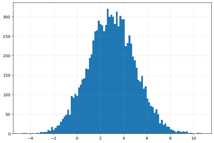
To draw from a more general \(\N(\mu,\sigma^2)\) distribution, we use the normal method. Here, we use \(\mu=3\) and \(\sigma=2\). (Note that the function takes the argument \(\sigma\), not \(\sigma^2\).)
draws2 = rng.normal(3, 2, 10000)

draws2.mean(), draws2.std()
(2.977375721852533, 2.0122793644789576)
Here is a histogram of the simulated values. Not surprisingly, it follows the typical shape of a normal distribution, although with some random noise.
import matplotlib.pyplot as plt

fig, ax = plt.subplots(figsize=(9,6))
ax.hist(draws2, bins=100)
ax.grid(alpha=0.25)
plt.show()
Specifying a seed#
Algorithms to generate pseudorandom numbers use a seed as a starting point to generate the next number in the sequence. As each random number is generated, the state of the algorithm changes, allowing it to generate new random draws. We can think of the pseudorandom number generator as creating an infinite series of numbers, and by providing a seed we choose where in the series to begin.
If we don’t provide a seed to the algorithm, the current time is used to generate one. However, if we want to generate a stream of reproducable random numbers, we can specify a seed, which will allow us to get the same random numbers again.
# providing a seed as an argument
rng = np.random.default_rng(8675309)

# random draws
rng.standard_normal((5,3))
array([[-0.03940941,  0.70927967, -0.00996881],
       [ 0.57052593, -0.32324939,  2.16436963],
       [ 1.62858142,  0.03537361, -0.59590844],
       [ 1.42716144,  1.95400359,  1.69854378],
       [ 0.11976012, -0.98484949,  0.13702581]])
If we now provide the same seed again, we’ll get the same random draws.
rng = np.random.default_rng(8675309)

rng.standard_normal((5,3))
array([[-0.03940941,  0.70927967, -0.00996881],
       [ 0.57052593, -0.32324939,  2.16436963],
       [ 1.62858142,  0.03537361, -0.59590844],
       [ 1.42716144,  1.95400359,  1.69854378],
       [ 0.11976012, -0.98484949,  0.13702581]])
Using scipy#
Many statistical functions are also available in the SciPy library.
import scipy.stats as scs
Here we use norm to denote the normal distribution, and call the rvs method to draw random variables.
scs.norm(5,10).rvs(size=(5,3))
array([[ -0.6152847 ,  10.19143968,  14.98697678],
       [ 13.1856673 ,   8.45870031,   2.25839151],
       [  3.10615868,   4.87658343,  -7.0636507 ],
       [  3.45013598,   8.19192563, -11.62850981],
       [ -9.7026336 ,  14.34620526,  -3.1529454 ]])
We can specify a state as follows. Even though we’re working in scipy, we specify the state of the random number generator within numpy. The two modules work very closely with each other.
rng = np.random.RandomState(8675309)

scs.norm(0,1).rvs(size=(5,3), random_state=rng)
array([[ 0.58902366,  0.73311856, -1.1621888 ],
       [-0.55681601, -0.77248843, -0.16822143],
       [-0.41650391, -1.37843129,  0.74925588],
       [ 0.17888446,  0.69401121, -1.9780535 ],
       [-0.83381434,  0.56437344,  0.31201299]])
# reset seed, verify that draws are the same
rng = np.random.RandomState(8675309)

scs.norm(0,1).rvs(size=(5,3), random_state=rng)
array([[ 0.58902366,  0.73311856, -1.1621888 ],
       [-0.55681601, -0.77248843, -0.16822143],
       [-0.41650391, -1.37843129,  0.74925588],
       [ 0.17888446,  0.69401121, -1.9780535 ],
       [-0.83381434,  0.56437344,  0.31201299]])
Population Moments vs. Sample Moments#
It is worth pausing to think about the difference between the following two lines of code:
scs.norm(3,2).mean()
3.0
scs.norm(3,2).rvs(100).mean()
3.1114116301634205
These two lines do very different things, even though they look similar.
The first line computes the theoretical (or population) mean of a normal distribution with \(\mu=3\) and \(\sigma=2\). Because the mean of a normal distribution is just its parameter \(\mu\), this will always return exactly 3—there’s no randomness involved. It is a theoretical quantity, derived by applying math to the definition of the probabibility density function for a normal distribution.
The second line of code first draws 100 random observations from that same normal distribution, then computes the sample mean of those draws. Because the data are a random sample, this value will not be exactly 3, but it should be close to 3, and it will change slightly each time you run the code (unless you fix a random seed).
The scipy package has many theoretical properties of distributions built in. For example, we can calculate the theoretical skewness and excess kurtosis of a distribution:
# Create a theoretical binomial distribution

b = scs.binom(n=10, p=0.4)
# specify "s" for skewness and "k" for kurtosis

pop_skew = b.stats(moments='s')
pop_kurt = b.stats(moments='k')

print(f"Population skewness: {pop_skew:.4f}")
print(f"Population kurtosis: {pop_kurt:.4f}")
Population skewness: 0.1291
Population kurtosis: -0.1833
And we can compare these to the corresponding values in a sample of 100,000 draws. We should find that they are quite close to the population values.
draws = b.rvs(100000)

smpl_skew = scs.skew(draws)
smpl_kurt = scs.kurtosis(draws)

print(f"Sample skewness: {smpl_skew:.4f}")
print(f"Sample kurtosis: {smpl_kurt:.4f}")
Sample skewness: 0.1301
Sample kurtosis: -0.1922