Probability theory

To begin developing a theory of probability, it is useful to consider a simple random process such as a flipping a coin. There are two possible outcomes of a single coin toss, “Heads” or “Tails,” which we’ll denote \(H\) and \(T\), respectively.

The sample space is almost always denoted with the Greek letter \(\Omega\) (upper-case Omega). Perhaps this is a reference to the biblical book of Revelation, when God says “I am Alpha and Omega, the beginning and the end.” (Revelation 21:6) The “end” here is the set of all possible things that can happen.

The sample space is the set of possible outcomes:

\[\Omega = \{H, T\},\]

indicating that one of these two events must occur.

A coin flip is an example of a random process that has two possible outcomes, called a Bernoulli trial, where the probability of the event occuring is given by \(p\) (and, obviously, of it not occuring by \(1-p\)). If a coin is fair, the probability of Heads (or, equivalently, of Tails) is \(p=0.5\).

Examples of binary outcomes that can be modeled as Bernoulli trials include:

• a single coin flip comes up Heads;

• a customer chooses whether to buy a product;

• a company declares bankruptcy next week; or

• a stock price increases in the next 15 seconds.

Each outcome \(\omega \in \Omega\) has an associated probability, given by the probability measure \(\P: \Omega \rightarrow [0,1]\). For a fair coin flip,

\[\P(H) = \P(T) = \frac{1}{2}.\]

To be sensible, the probability measure must be defined such that the probability that some event in the sample space occuring is 1, so

\[\P(\Omega) = \sum_{\omega\in\Omega} \P(\omega) = \P(H) + \P(T) = 1.\]

In other words, the probability that something happens is one. As a matter of logic, if that weren’t true, we would have to redefine the sample space. If it is correctly defined as the exhuastive set of all possible outcomes, then one of those outcomes must occur.

Random variables

A random variable is a function that maps an event to a real number. For example, define the random variable \(X\) to be the number of Heads that we observe in a single coin flip,

\[\begin{equation*} X(\omega) = \left\{\begin{matrix} 0 & \quad \omega = T,\\ 1 & \quad \omega = H. \end{matrix}\right. \end{equation*}\]

This says simply that if the event \(\omega=T\) occurs then \(X=0\), and if the event \(\omega=H\) occurs then \(X=1\). In general, a random variable (“RV”) maps from an event space to some real number: \(X\!: \Omega \rightarrow \mathbb{R}\).

We can then apply the probability measure to \(X\). For some \(x\in \mathbb R\),

\[\P(X = x) := \P(\{\omega\in\Omega: X(\omega)=x\}).\]

In words, this says simply that the probability that the random variable \(X\) takes on a value of \(x\) is equal to the probability that an outcome \(\omega\) occurs that causes \(X\) to equal \(x\). Therefore,

\[\begin{align*} \P(X=0) &= \P(\omega=T) = \tfrac{1}{2}, \\ \P(X=1) &= \P(\omega=H) = \tfrac{1}{2}. \end{align*}\]

It is common practice to write simply \(\P(x)\) rather than \(\P(X=x)\).

More generally, a random variable defined for a Bernoulli trial with probability \(p\) is

(9)\[\begin{split}\begin{align} \P(X=1) &= p, \\ \P(X=0) &= 1-p. \end{align}\end{split}\]

The event that leads to \(X=1\) is often called “success.”

Let’s apply the same framework to an experiment where we flip a coin twice. As before, the sample space is the set of possible outcomes:

\[\Omega = \{HH, HT, TH, TT\}.\]

The probability measure is

\[\P(HH) = \P(HT) = \P(TH) = \P(TT) = \frac{1}{4}.\]

As expected, \(\P(\Omega) = 1.\) Again, define the random variable \(X\) to be the number of Heads that we observe in our two coin flips,

\[\begin{equation*} X(\omega) = \left\{\begin{matrix} 0 & \omega = TT,\\ 1 & \omega = \{HT, TH\},\\ 2 & \omega = HH. \end{matrix}\right. \end{equation*}\]

Applying the probability measure to \(X\),

\[\begin{align*} \P(X=0) &= \P(\omega=TT) = 1/4, \\ \P(X=1) &= \P(\omega=HT) + \P(\omega=TH) = 1/2, \\ \P(X=2) &= \P(\omega=HH) = 1/4. \end{align*}\]

Formally, an event is any subset of \(\Omega\). For example, the event that at least one of the flips is Heads is

\[E = \{HH, HT, TH\}.\]

The probability of this event is the sum of the probabilities of each element in the event,

\[\begin{align*} \P(E) &= \P(HH) + \P(HT) + \P(TH) \\ &= 3\times\frac{1}{4} \\ &= 0.75. \end{align*}\]

Exercise

Suppose you roll a single six-sided die. Define the random variable \(X\) to be the number shown on the die. What is the sample space? What are the probabilities associated with each possible value of the \(X\)?

Extra credit

Modern probability theory, introduced in the 1930s by Andrey Kolmogorov, is formally defined using a probability space \((\Omega, \mathcal{F}, \P)\), where \(\mathcal{F}\) is the set of all possible events is (called the event space or the “\(\sigma\)-algebra”). In the two-flip example, this is

\[\mathcal{F} = \{\emptyset, HH, HT, TH, TT, \{HH, HT\}, \{HH, HT\}, \ldots, \{HH, HT, TH, TT\} \}.\]

In this example, \(\Omega\) is countable, so \(\mathcal{F}\) is the power set of \(\Omega\), and its cardinality (the number of elements in the set) is \(2^4=16\). More generally, though, the sample space need not be countable, and a different \(\sigma\)-algebra must be used. A nice introduction to these ideas may be found on Wikipedia.

Binomial distribution

Generalizing from two coin flips, suppose that we repeat a Bernoulli trial \(n\) times. The trials are assumed to be mutually independent, meaning that the outcome of each trial has no effect on any other outcomes. Let \(X\) equal the number of Heads out of these trials. We characterize the random variable \(X\) by determining \(\P(X=k)\) for any possible value of \(k\). This is given by the probability mass function (PMF),

\[f(k; n,p) := \P(X=k) = {\binom {n}{k}}p^{k}(1-p)^{n-k}, \quad k=0,1,2,\ldots,n.\]

A random variable with this PMF has a Binomial distribution, which we write as \(X \sim B(n,p)\).

Exercise

Show that when \(n=1\) this PMF reduces to probability function for a Bernoulli trial.

Solution

We have

\[f(0; p) = {\binom {1}{0}}p^{0}(1-p)^{1-0} = 1-p,\]

and

\[f(1; p) = {\binom {1}{1}}p^{1}(1-p)^{1-1} = p,\]

which matches the function in (9).

The PMF for the Binomial distribution (along with many others) is available in the scipy module. Here we calculate \(f(k; 3, 0.5)\) for each possible \(k\).

n = 3    # number of trials
p = 0.5  # probability of success in each trial

scs.binom.pmf([0, 1, 2, 3], n, p)

array([0.125, 0.375, 0.375, 0.125])

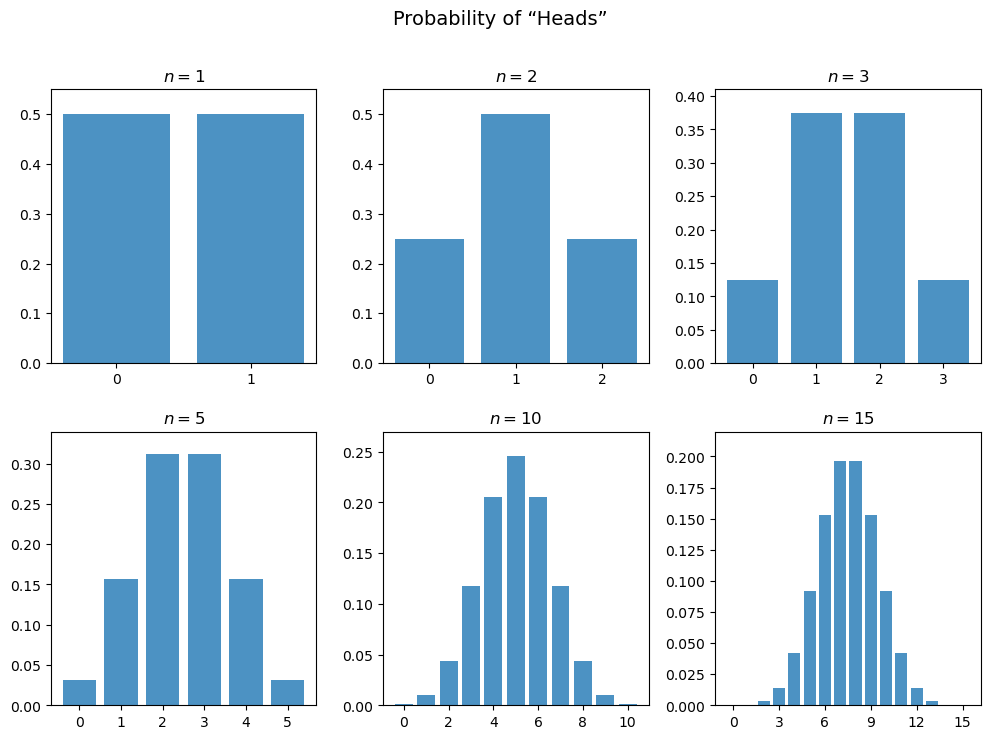
As we increase \(n\), the probabilities associated with each outcome change, and so does the shape of the PMF.

Show code cell source

Hide code cell source

ntrials = [1, 2, 3, 5, 10, 15]

fig, axes = plt.subplots(2, 3, figsize=(12, 8))
fig.suptitle('Probability of “Heads”', fontsize=14)
plt.subplots_adjust(hspace=.25, wspace=0.25)
for n,ax in zip(ntrials, axes.ravel()):
    domain = np.arange(n+1)
    probs = scs.binom(n, 0.5).pmf(domain)
    ax.bar(domain, probs, alpha=0.8, align='center')
    ax.set(title=f'$n = {n}$',
           ylim=(0, np.round(probs.max()*1.1,2)),
           xticks=np.arange(n+1).astype(int) if n<10 else np.arange(0,n+1,n/5).astype(int))

plt.show()

Expected value and variance

The expected value or expectation of a discrete random variable \(X\) with possible outcomes \((x_1, x_2, \ldots, x_n)\) is the weighted average of the outcomes,

\[\begin{equation*} \E(X) := \sum_{\omega\in\Omega} \P(\omega)\, X(\omega) = \sum_{i=1}^n \P(x_i)\, x_i. \end{equation*}\]

The expected value, often denoted by the Greek letter \(\mu\), measures the location or central tendency of the distribution.

For example, suppose we flip a fair coin 3 times, and assign to \(X\) the number of times Heads comes up, so \(X\sim B(3,0.5)\). The sample space is

\[\Omega = \{TTT, TTH, THT, HTT, THH, HTH, HHT, HHH\},\]

so the random variable \(X\) has these possible values:

\[\begin{equation*} X = \left\{\begin{matrix} 0 & \text{with probability } 1/8,\\ 1 & \text{with probability } 3/8,\\ 2 & \text{with probability } 3/8,\\ 3 & \text{with probability } 1/8.\\ \end{matrix}\right. \end{equation*}\]

The expectation of \(X\) is therefore

\[\begin{align*} \E(X) &= \P(X=0) \cdot 0 + \P(X=1) \cdot 1 + \P(X=2) \cdot 2 + \P(X=3) \cdot 3 \\ &= \frac{1}{8} \cdot 0 + \frac{3}{8} \cdot 1 + \frac{3}{8} \cdot 2 + \frac{1}{8} \cdot 3 \\ &= 1.5 \end{align*}\]

As this example makes clear, the expected value of \(X\) need not be a value from any outcome in its sample space.

Key fact

The expecation of a random variable is the average of the population. For a random process like rolling a die, this is the average we would get if we could repeat the process infinitely many times.

The variance of \(X\) is a measure of how much the probability mass is spread out around its expected value. It is defined as the weighted sum of the squared deviations from the expected value,

\[\var(X) := \E[(X-\E(X))^2] = \sum_{i=1}^n \P(x_i)(x_i-\E(X))^2.\]

The variance is typically denoted by \(\sigma_X^2\). Its square-root, \(\sigma_X\), is the standard deviation of the distribution.

Continuing to define \(X\) as above, we have

\[\begin{align*} \var(X) &= \P(X=0) \cdot (0-1.5)^2 + \P(X=1) \cdot (1-1.5)^2 + \P(X=2) \cdot (2-1.5)^2 + \P(X=3) \cdot (3-1.5)^2 \\ &= \frac{1}{8} \cdot 2.25 + \frac{3}{8} \cdot 0.25 + \frac{3}{8} \cdot 0.25 + \frac{1}{8} \cdot 2.25 \\ &= 0.75 \end{align*}\]

The scipy module provides the expected value (also called the mean), variance, and standard deviation of a random variable given the parameters of its distribution.

B = scs.binom(3, 0.5)

print(B.mean())
print(B.var())
print(B.std())

1.5
0.75
0.8660254037844386

Exercise

Find the expected value and variance of a Bernoulli random variable.

Solution

Using the defition of expectation and variance,

\[\begin{align*} \E(X) &= \P(0) \times 0 + \P(1) \times 1\\ &= (1-p) \times 0 + p \times 1 \\ &= p \end{align*}\]

\[\begin{align*} \var(X) &= \P(0) \times (0-p)^2 + \P(1) \times (1-p)^2 \\ &= (1-p)p^2 + p(1-p)^2 \\ &= p(1-p)(p+1-p) \\ &= p(1-p) \end{align*}\]

The following code uses assert to verify that a boolean expression is True; if it isn’t, an exception is raised. These conditions are all true, so the code executes without raising any exceptions.

for p in [0.1, 0.4, 0.99]:
    assert scs.bernoulli(p).mean() == p
    assert scs.bernoulli(p).var() == p*(1-p)

Linearity of expectations

We saw above that the mean and variance of a distribution are defined using the expectations operator \(\E\) which we redefine here as applying to any function \(g(\cdot)\) of the random variable \(X\),

\[\E(g(X)) = \sum_{\omega\in\Omega} \P(\omega)\, g(X(\omega)).\]

In the simplest case that we previously considered, \(g(x)=x\). It follows immediately that, for any constant \(a\),

\[\E(a) = \sum_{\omega\in\Omega} \P(\omega)\, a = a \sum_{\omega\in\Omega} \P(\omega) = a.\]

This holds for any nonrandom — also called nonstochastic — variable. In other words, if \(a\) doesn’t depend on the outcome \(\omega\) then its value isn’t random, and its expectation is just \(a\).

Exercise

Find the variance of a constant \(a\).

Solution

Applying the definition of variance,

\[\begin{equation*} \var(a) = \E(a - \E(a))^2 = \E(a-a)^2 = \E(0)^2 = 0. \end{equation*}\]

Not surprisingly, \(a\) has no variance — it’s constant!

More generally, we can show that the expectations operator \(\E\) is linear. Let \(Z=a+bX\) for some constants \(a\) and \(b\). Then

\[\E(Z) = \E(a+bX) = a + b\E(X).\]

Exercise

Use the definition of the \(\E\) operator to show that if \(X\) and \(Y\) are two random variables then

\[\E(a + bX + cY) = a + b\,\E(X) + c\, \E(Y)\]

for two arbitrary constants \(a\), \(b\), and \(c\). (Note that when we say \(X\) and \(Y\) are two random variables, we mean that they are both functions of elements of the same outcome space \(\Omega\).)

The variance, however, is not linear:

\[\begin{align*} \var(Z) &= \E[(Z-\E(Z))^2] \\ &= \E[(a+bX-a-b\E(X))^2] \\ &= \E[(b(X-\E(X)))^2] \\ &= \E[b^2(X-\E(X))^2] \\ &= b^2 \; \E[(X-\E(X))^2] \\ &= b^2 \var(X). \end{align*}\]

In particular, this implies that

\[\var(-X) = \var(X),\]

which is especially important when we calculate the volatility of portfolios that include short positions.

Key fact

We can use these facts to shift and rescale a random variable.

For example, suppose we have a random variable \(X\) with \(\E(X)=0\) and \(\var(X)=1\). If we create a new random variable

\[ Y=\mu + \sigma X, \]

then \(\E(Y) = \mu\) and \(\var(Y) = \sigma^2\). We have shifted the mean by \(\mu\) and rescaled it to have a variance of \(\sigma^2\).

Key fact

The linearity of the expectations operator allows us to write variance conveniently as

\[\begin{align*} \var(X) &= \E[X^2 - 2X\E(X) + \E(X)^2] \\ &= \E[X^2] - 2\E(X)\E(X) + \E(X)^2 \\ &= \E(X^2) - \E(X)^2. \end{align*}\]

Exercise

The random variable \(Y\) follows a Binomial distribution with parameters \(n\) and \(p\). Find \(\E(Y)\) and \(\var(Y)\).

Solution

Since \(Y\sim B(n,p)\), it is the sum of \(n\) independent Bernoulli trials. We saw previously that if \(X\) has a Bernoulli distribution then \(\E(X)=p\) and \(\var(X)=p(1-p)\). Therefore,

\[\E(Y) = \E\left(\sum_{i=1}^n X_i\right) = \sum_{i=1}^n \E(X_i) = n \cdot \E(X) = np,\]

and

\[\var(Y) = \var\left(\sum_{i=1}^n X_i\right) = \sum_{i=1}^n \var(X_i) = n\cdot \var(X) = np(1-p).\]

The first result is quite intuitive: If we flip a fair coin \(n\) times, we would expect it to come up Heads \(0.5\times n\) times. But of course it might turn up Heads more or less than that. The variance, in this case \(0.25\times n\), tells us how variability we can expect in the outcome. We will soon delve into this more deeply.

Note also that the calculation of the variance here is correct only because we assumed that the the Bernoulli trials are independent; that is, the outcome of each trial has no effect on the outcomes of other trials. If the trials are related in some way, these calculations no longer hold, as we’ll see when we discuss covariance.

The normal distribution

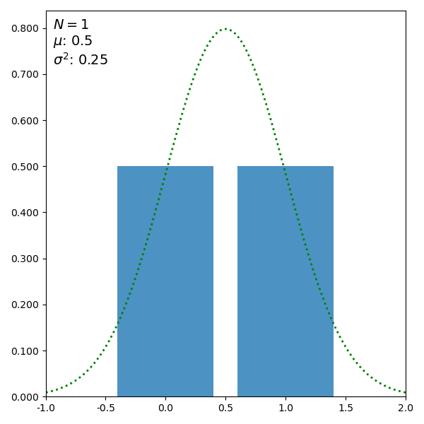
Consider what happens as we increase the number of trials. The figure shows the distribution of outcomes according to the binomial distribution along with a continuous function called the normal distribution. (Move the slider to increase \(N\).)

Number of trials: 1  

In particular, suppose \(n=50\), so \(\E(X)=25\) and \(\var(X)=12.5\).

Some intuition for the connection between the Binomial distribution and the normal distribution can be gained by considering a Galton Board, demonstrated nicely in this Youtube video.

Show code cell source

Hide code cell source

fig, ax = plt.subplots(figsize=(8,5))

n = 50

# Binomial PMF
domain = np.arange(n+1)
probs = scs.binom(n, 0.5).pmf(domain)
ax.bar(domain, probs, alpha=0.8, align='center', label='$B({},{})$'.format(n,p))

# Normal density function
μ = n*p
σ = np.sqrt(n*p*(1-p))
x = np.linspace(0, n, 250)
pdf = scs.norm.pdf(x, μ, σ)
ax.plot(x, pdf, 'g:', linewidth=1, label=r'$\mathcal{N}$' + '({:.0f},{:.1f})'.format(μ,σ**2))

ax.grid(alpha=0.3)
ax.legend(loc='upper left')
ax.set_xlim(10,40)
plt.show()

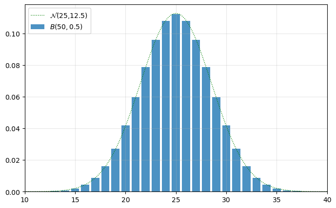
The fit of this curve to the binomial distribution is very good — the line and bars match exactly for most values of \(X\). As \(n\) increases, the fit continues to get better; in the limit, the binomial distribution converges to the normal distribution.

The normal distribution is also called the “Gaussian distribution” for Carl Friedrich Gauss, one of the most important mathematicians of all time. Gauss is pictured in this German banknote along with the normal density function.

In contrast to the binomial distribution, which is only defined over discrete values \(k=\{0, 1, \ldots, n\}\), the normal distribution is a continuous distribution, defined over the entire real line. Like all such continuous distributions, it is characterized by a probability density function (PDF) that is defined over a continuous domain. (In the graphs above, we’re only plotting the distribution over the same domain as the binomial distribution, but the normal PDF is actually defined everywhere.)

The PDF for a random variable \(X\) with a normal distribution, which we write as \(X \sim \N(\mu,\sigma^2)\), is given by

\[f_X(x; \mu, \sigma)={\frac {1}{\sigma {\sqrt {2\pi }}}}\exp\left\{-{\frac {1}{2}}\left({\frac {x-\mu }{\sigma }}\right)^{2}\right\}.\]

Note

It is easy to get confused by the difference between \(\E(X)\) and \(\mu\). As we have seen, \(\E(X)\) is the expected value of the random variable \(X\), regardless of what kind of random variable it is. It is a number we calculate by applying the expectations operator \(\E\) to the random variable.

If we calculate an expected value of a random variable with the Normal distribution, \(X\sim\N(\mu, \sigma^2)\), using the method explained below, we will find that

\[\E(X) = \mu.\]

That is, when a random variable has the pdf \(f_X(x; \mu, \sigma)\) shown above, it just so happens that the expected value of this random variable is equal to the parameter value \(\mu\).

Since the normal distribution is so important and pervasive, its expected value \(\mu\) is often used as a general symbol for the more general concept of \(\E(X)\). But, as we will soon see, there are many random variables where the expected value is not a simple parameter of their distribution. It just happens to be true with normally-distributed random variables.

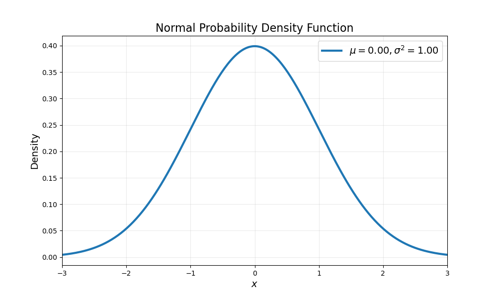
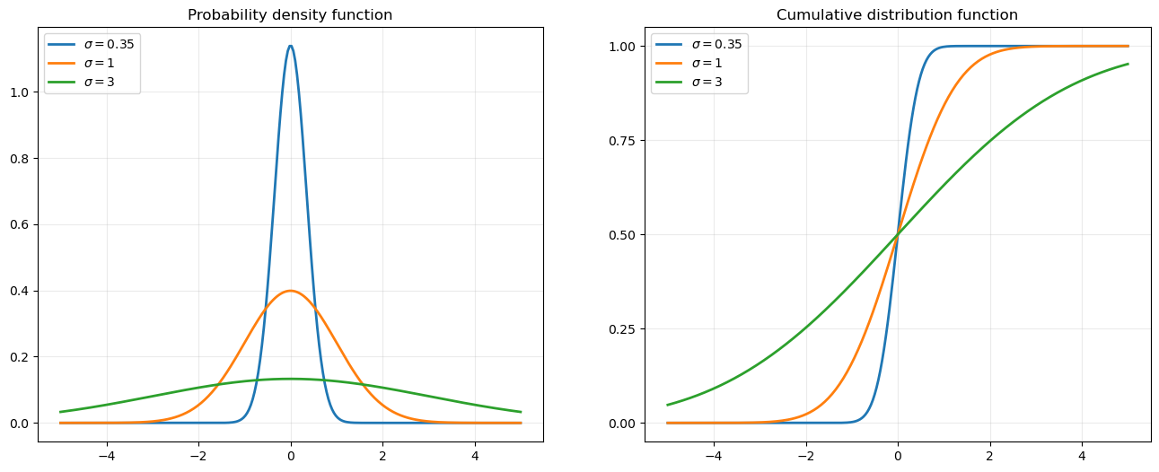
The parameters \(\mu\) and \(\sigma\) control the location and shape of the distribution. With \(\mu=0\) and \(\sigma=1\), we have the “standard” normal distribution, \(X \sim \N(0,1)\), with density

\[f_X(x)={\frac {1}{\sqrt {2\pi }}} e^{\frac{-x^2}{2}}.\]

Show code cell source

Hide code cell source

fig, ax = plt.subplots(figsize=(10,6))

xlims = (-3, 3)
x = np.linspace(*xlims,250)
for μ,σ in [(0,.5), (0,1), (0,2), (-2,1)]:
    ax.plot(x, scs.norm.pdf(x, loc=μ, scale=σ), lw=3,
            label=r'$\mu={}, \sigma^2={}$'.format(μ,σ**2))

ax.legend(prop={'size': 14})
ax.grid(alpha=0.25)
ax.set_ylabel('Density', size=14)
ax.set_xlabel('$x$', size=14)
ax.set_title('Normal Probability Density Function', size=16)
ax.set_xlim(xlims)

plt.show()

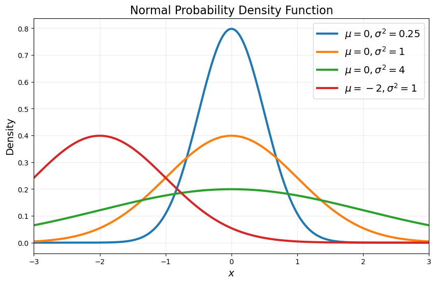
You can try different combinations of parameters to see how the shape and center of the distribution shift:

μ=0.00   σ=1.00

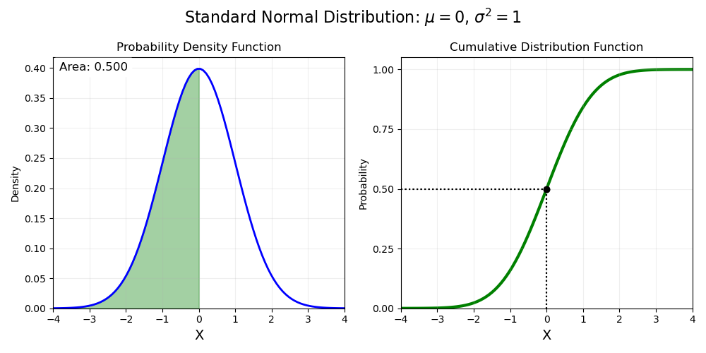
Rather than directly giving probabilities, the PDF is a tool for calculating the probability. In particular, we integrate under the curve to find the cumulative distribution function (CDF), which gives the probability that the random variable \(X\) is less than a given value \(x\):

\[F_X(x) := \P(X\leq x) = \int_{-\infty}^x f_X(z)\,dz.\]

The CDF and PDF of a normal distribution are often written as \(\Phi(x)\) and \(\phi(x)\), respectively.

Select a value for \(x\): 0.0  

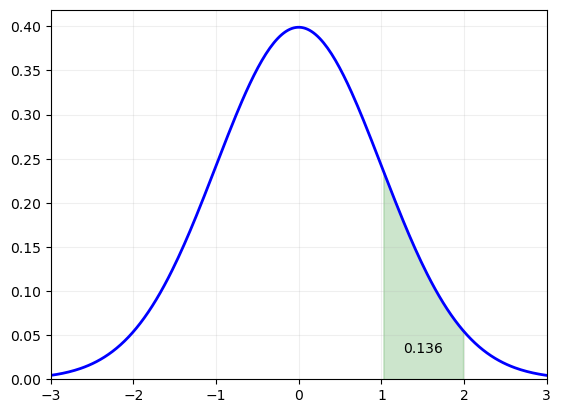
We can calculate the probability that \(X\) is between \(a\) and \(b\) (with \(a<b\)) by calculating

\[\P(a<X<b) = F_X(b) - F_X(a) = \int_a^{b} f_X(x)\,dx.\]

For example, the probability that a random draw of \(X\sim \N(0,1)\) will be between 1 and 2 is:

area = scs.norm().cdf(2) - scs.norm().cdf(1)
print(area)

0.13590512198327787

Show code cell source

Hide code cell source

fig, ax = plt.subplots()

# plot pdf
px = scs.norm.pdf(x)
ax.plot(x, px, 'b-', lw=2)

# fill area under the curve between x=1 and x=2
mask = (x > 1) & (x < 2)
ax.fill_between(x[mask], px[mask], color='g', alpha=0.2)

ax.text(1.5, 0.03, f'{area:0.3f}', horizontalalignment='center')

ax.grid(alpha=0.2)
ax.set_xlim(xlims)
ax.set_ylim(0, None)

plt.show()

A valid CDF must have the following properties:

• \(F(x)\) is non-decreasing, meaning that \(f(x)\geq 0\) for all \(x\);

• \(0\leq F(x)\leq 1\); and

• \(F(-\infty)=0\) and \(F(\infty)=1\).

Intuitively, \(F(\infty)=1\) because the probability that \(X\) will be less than infinity must be one: \(X\) has to have a realization somewhere on the real line. For the same reason, \(F(-\infty)=0\).

The fact that \(F(\infty)=1\) explains why we divide by \(\sqrt{2\pi}\) in the normal density function; it is simply a normalizing constant to force the probability to be one in the limit. To see why this is the necessary constant, refer to our previous discussion of the Gaussian integral.

Warning: A PDF is not a ``probability function’’

There are two important facts about probability density functions that may seem surprising at first:

• \(f(x)\) does not give the probability of \(x\). It is simply an input to the calculation of the probability of a possible outcome.

• Since \(f(x)\) is not a probability, there is no reason that it must be less than 1. It must, however, never be negative. (Using the sliders above, you can find values of \(\sigma\) that will make the density function have values greater than one.)

Perhaps most surprising is the fact that \(\P(X=x)=0\) for any \(x\). Yes, you read that right: the probability that \(X\) takes on any particular value is zero. We can see this by using the definition of the CDF:

\[\P(X=x) = \P(x\leq X\leq x) = F(x) - F(x) = 0.\]

Ituitively this is because there are an infinite number of outcomes so the probability of any one of them is \(\frac{1}{\infty} = 0\).

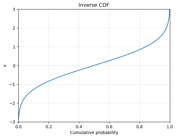
Inverse CDF

The inverse of the CDF function allows us to answer the question “what value of a random draw from \(X\) would have a probability of less than \(p\) of happening?”. Rather than giving the probability associated with a realization of the random variable, it gives us what realization would be a associated with a given level of probability. In SciPy, the ppf function (“percent point function”) gives these values.

p = np.array([0.005, 0.01, 0.025, 0.05, 0.5, 0.95, 0.975, 0.99, 0.995])

pd.DataFrame({
    'probability': p,
    'value': scs.norm().ppf(p)}
).set_index('probability')

	value
probability
0.005	-2.575829
0.010	-2.326348
0.025	-1.959964
0.050	-1.644854
0.500	0.000000
0.950	1.644854
0.975	1.959964
0.990	2.326348
0.995	2.575829

That is, there is a 2.5% chance that a draw from a standard normal distribution would have a value of less than –1.96. Because the distribution is symmetric, there is also a 2.5% chance that the draw would be greater than 1.96 (that is, there’s a 97.5% that it would be less than 1.96). We will revisit these well-known “critical values” when we discuss parameter estimation.

Show code cell source

Hide code cell source

ps = np.linspace(0,0.999,500)

fig, ax = plt.subplots()
ax.plot(ps, scs.norm().ppf(ps))

ax.grid(alpha=0.3)
ax.set_xlim(0,1)

ax.set_ylabel('$x$')
ax.set_xlabel('Cumulative probability')
ax.set_title('Inverse CDF')

ax.set_ylim(xlims)

plt.show()

Expected value of continuous RVs

The expected value of a continuous random variable is defined analagously to the defintion above for the discrete case:

\[\E(X) := \sum_{\omega\in\Omega} \P(\omega)\, X(\omega) = \int_{-\infty}^{\infty} f_X(x) x \, dx.\]

Again, it is simply the weighted average of all possible values of \(x\). The only difference is that we calcualate the probability over the entire real line, and we use the PDF instead of the PMF.

Similarly, the variance of a continuous random variable is

\[\var(X) := \int_{-\infty}^{\infty} f_X(x) (x-\E(X))^2 \, dx.\]

As noted above, it can be shown for the normal distribution that the two parameters of the density function, \(\mu\) and \(\sigma^2\), are equal to the expected value and variance of the distribution, \(\E(X)\) and \(\var(X)\), respectively.

Exercise

The code below uses quadrature to calculate the integral for the expected value of \(X\sim\N(\mu,\sigma)\). If you change the parameter μ and run the code, you will find that the integral is always equal to whatever value of μ you chose. This should convince you that the expected value is, in fact, \(\mu\).

from scipy.integrate import quad

# Parameters for the normal distribution
μ = 3.5
σ = 1

# Define the PDF of the normal distribution
def normal_pdf(x, μ, σ):
    return (1 / (σ * np.sqrt(2 * np.pi))) * np.exp(-0.5 * ((x - μ) / σ) ** 2)

# Define the function to integrate
def pdf_times_x(x, μ, σ):
    return x * normal_pdf(x, μ, σ)

# Integrate the function from -∞ to ∞
result, error = quad(pdf_times_x, -np.inf, np.inf, args=(μ, σ))

print(f"Integral result: {result:0.4f}, with error estimate: {error:0.2e}")

Another way to do the same kind of exercise is to confirm that the theoretical expected value (``mean’’) and variance reported by scipy equals what we expect, which is what this code does:

for μ in [-1, 0, 1]:
    for σ in [0.5, 2, 4]:
        X = scs.norm(μ,σ)
        assert (X.mean() == μ) and (X.var() == σ**2)

Make sure you understand the following:

• What does scs.norm(μ,σ) do?

• What calculation is happening when we call X.mean() and X.var()? Specifically, can you point to an equation somewhere on this page that is being calculated?

• What does assert do in this code?

This fact—and that the normal distribution is so important throughout statistics—is of course the reason that we use the symbols \(\mu\) and \(\sigma^2\) both for the parameters of the probability distribution and as general symbols for mean and variance.

As \(\sigma\) increases, both the PDF and CDF becomes flatter to reflect the greater probability of a wider range of outcomes.

Show code cell source

Hide code cell source

fig, (ax1, ax2) = plt.subplots(1, 2, figsize=(16,6))

x = np.linspace(-5, 5, 250)

for σ in [0.35, 1, 3]:
    ax1.plot(x, scs.norm.pdf(x, scale=σ), lw=2, label=r'$\sigma={}$'.format(σ))
    ax2.plot(x, scs.norm.cdf(x, scale=σ), lw=2, label=r'$\sigma={}$'.format(σ))

for ax in (ax1, ax2):
    ax.legend(loc='upper left')
    ax.grid(alpha=0.25)

ax1.set_title('Probability density function')
ax2.set_title('Cumulative distribution function')
ax2.set_yticks([0, .25, .5, .75, 1])
plt.show()

Exercise

Make a plot like the one above to show how the PDF and CDF shift to the left or right as we change \(\mu\).

Higher-order moments

The expected value is also called the first moment of \(X\). More generally, the \(k\)th moment is \(\E(X^k)\).

Central moments are defined around the mean. For example, variance is the second central moment:

\[\var(X) = \E\left[(X - \E(X))^2\right].\]

Higher-order moments can be similarly defined; the \(k\)th central moment is

\[\mu_k := \E\left[(X-\E(X))^k\right]=\int_{-\infty }^{\infty }(x-\E(X))^k f(x)\, dx.\]

Extra credit

Use properties of \(f_X(x)\) to show that \(\mu_0 = 1\) and \(\mu_1\) = 0.

The skewness and kurtosis are, respectivley, the third and fourth standardized moments — that is, the central moment divided by the standard deviation to make the ratio unitless:

\[\begin{align*} \operatorname{Skew}[X] &:= \E\left[\left({\frac {X-\E(X) }{\sqrt{\var(X)} }}\right)^3\right]={\frac {\E \left[(X-\E(X) )^3\right]}{\sigma^3}} = {\frac {\mu_{3}}{\sigma^{3}}}, \\ \operatorname{Kurt}[X] &:= \E \left[\left({\frac {X-\E(X) }{\sqrt{\var(X)} }}\right)^{4}\right]= \frac{\E \left[(X-\E(X) )^{4}\right]}{\sigma^4} = \frac {\mu_4}{\sigma^4}. \end{align*}\]

These moments are all helpful in characterizing what a distribution “looks like.” The mean tells us where the center of the distribution is; the variance measures the dispersion around the mean; the skewness describes the asymmetry of the distribution; and kurtosis measures how “thick” its tails are.

The skewness of a normal distribution is 0. The kurtosis is 3, and because the normal distribution is so foundational, people usually refer to \(\operatorname{Kurt}[X]-3\) as simply the excess kurtosis.