A model of prices

A model of prices#

Consider the following simple model for how the price of an asset can change over time. At time 0, the prices is \(P_0\). Over the next period of time, the price can either increase or decrease by a fixed amount \(\Delta\). The probabilities of the increase or decrease are, respectively, \(\pi\) and \(1-\pi\).

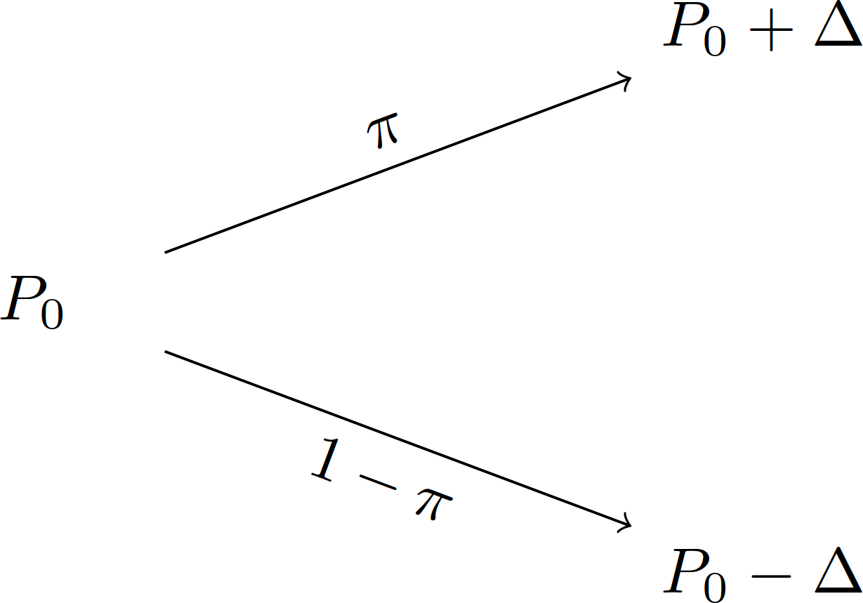
_images/Binomial_1.png — Fig. 2 One-period Binomial model.#

It’s easy to extend this model to allow for additional time intervals. After three intervals, we have:

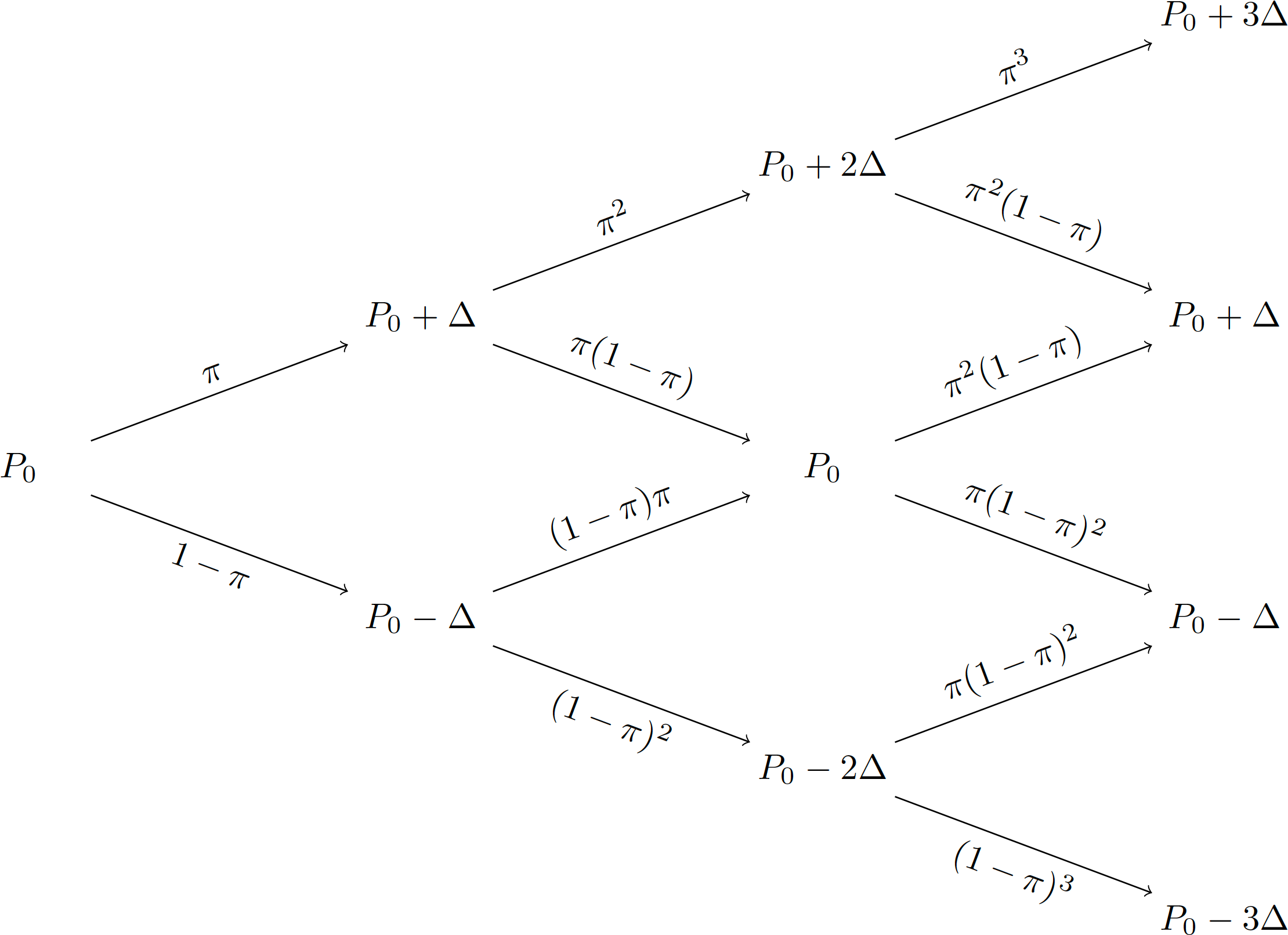
_images/Binomial_2.png — Fig. 3 Binomial model with 3 time periods.#

After three intervals there are four possible outcomes:

The price is \(P_0 + 3\Delta\). There is one path leading to this outcome: in every interval the price follows the high path, so this happens with probability \(\pi^3\).
The price is \(P_0 +\Delta\). There are three paths that lead to this outcome: a combination of two up moves and one down move. The probability of following each one of these paths is \(\pi^2(1-\pi)\).
The price is \(P_0 -\Delta\). Again, there are three paths leading to this outcome: any combination of one up move and two down moves, each of which has probability of \(\pi(1-\pi)^2\).
The price is \(P_0 -3\Delta\), which happens only if the price moves down in every period, implying a probability of \((1-\pi)^3\).

In general, after \(n\) periods, there will be \(n+1\) nodes. The number of paths to the \(k\)th terminal node (where we begin labelling the bottom node as “0”) is given by the binomial coefficient,

\[\binom {n}{k} = \frac{n!}{k!(n-k)!}, \quad k\in\{0, 1, \ldots, n\}.\]

The number of paths to the terminal nodes for varying values of \(n\) is shown below.

from scipy.special import binom

for n in [1, 3, 5, 10, 25]:
    print('{}:\t{}'.format(n, [int(binom(n, k)) for k in range(n+1)]))

[1, 1]
[1, 3, 3, 1]
[1, 5, 10, 10, 5, 1]
[1, 10, 45, 120, 210, 252, 210, 120, 45, 10, 1]
[1, 25, 300, 2300, 12650, 53130, 177100, 480700, 1081575, 2042975, 3268760, 4457400, 5200300, 5200300, 4457400, 3268760, 2042975, 1081575, 480700, 177100, 53130, 12650, 2300, 300, 25, 1]

The probability of arriving at node \(k\) is therefore

(7)#\[ \P(k) = {\binom {n}{k}}\pi^{k}(1-\pi)^{n-k}, \quad k=0,1,2,\ldots,n. \]

For example, setting \(\pi=0.5\), the probabilities associated with the four nodes in Fig. 3 are:

π = 0.5
n = 3
k = np.arange(n+1)

binom(3, k) * π**k * (1-π)**(n-k)

array([0.125, 0.375, 0.375, 0.125])

This function in equation (7) is called the probability mass function (PMF) for a binomial distribution. It gives the probability for each possible outcome of the random variable \(k\).

Rather than calculate the probability manually, we can call the pmf method from the SciPy stats library:

scs.binom.pmf(k, n, π)

array([0.125, 0.375, 0.375, 0.125])

Note

We are using two different functions called binom here. The first is scipy.special.binom which we imported and refer to as binom; this gives the binomial coefficent. The second is scipy.stats.binom, which is a class for calculating properties of the binomial distribution. While the two are related, they are conceptually distinct.

The price at terminal node \(k\) is

\[P_n = P_0 + (2k-n)\Delta.\]

For technical reasons, it is necessary to make \(\Delta\) depend on \(\pi\). Specifically, we set

\[\Delta = \sqrt{\pi(1-\pi)}.\]

Extra credit

In a standard binomial model, the price at each step can go up by \(u\) or down by \(d\), so after one period the price is either \(S_0 u\) or \(S_0 d.\) In the model above, we’re assuming that we have log-prices, so we add the price changes rather than multiplying.

Cox, Ross, and Rubinstein [1979] show that, for a tree to lead to a stock price with variance \(\sigma^2\), it must be that

\[u = e^{\sigma\sqrt{T/n}}.\]

In our model, \(\Delta = \ln(u)\), so

\[\Delta = \sigma\sqrt{T/n}.\]

Now, it can be shown that, in the limit, a binomial distribution converges to a Normal distribution with a mean of \(n\pi\) and variance of \(n\pi(1-\pi)\):

\[\frac{k-n\pi}{\sqrt{n\pi(1-\pi)}} \sim N(0,1).\]

Therefore,

\[\sigma = \sqrt{n\pi(1-\pi)}\]

and

\[\Delta = \sqrt{\pi(1-\pi)T}.\]

For simplification, we are assuming that \(T=1\).

Using the 3-period model from above, the table below shows for each node:

the number of “up” moves;
the number of “down” moves;
the net number of steps, \(\Delta\);
the number of possible paths leading to the node;
the price at that node; and
the probability of arriving at that node.

We assume that \(P_0=50\). With \(\pi=0.5\), we have \(\Delta=0.5\).

	n_up	n_down	Δs	paths	price	prob
node
0	0	3	-3	1	48.5	0.125
1	1	2	-1	3	49.5	0.375
2	2	1	1	3	50.5	0.375
3	3	0	3	1	51.5	0.125

Extending the model to 15 steps, we have:

	n_up	n_down	Δs	paths	price	prob
node
0	0	15	-15	1	42.5	0.000031
1	1	14	-13	15	43.5	0.000458
2	2	13	-11	105	44.5	0.003204
3	3	12	-9	455	45.5	0.013885
4	4	11	-7	1365	46.5	0.041656
5	5	10	-5	3003	47.5	0.091644
6	6	9	-3	5005	48.5	0.152740
7	7	8	-1	6435	49.5	0.196381
8	8	7	1	6435	50.5	0.196381
9	9	6	3	5005	51.5	0.152740
10	10	5	5	3003	52.5	0.091644
11	11	4	7	1365	53.5	0.041656
12	12	3	9	455	54.5	0.013885
13	13	2	11	105	55.5	0.003204
14	14	1	13	15	56.5	0.000458
15	15	0	15	1	57.5	0.000031

The expected value of \(P_n\) is the probability-weighted sum of all possible prices at time \(n\),

\[\E(P_n) = \sum_{k=0}^n \pi_k P^{(k)},\]

where \(P^{(k)}\) gives the price at terminal node \(k\). The expected value is often denoted by the Greek letter \(\mu\) (“mu”).

μ = (paths['prob'] * paths['price']).sum()

μ

50.000000000000014

Notice that the expected value is not a possible outcome: there is no path that ends with a price of 50. So while the mean might be one of the possible outcomes, there’s not guarantee that it will be.

Closely related to the expected value is the variance of \(P_n\). This is the probability-weighted sum of the squares of the difference between the price at each node and the expected value of \(P_n\):

\[\var(P_n) = \sum_{k=0}^n \pi_k \left(P^{(k)}-\E(P_n)\right)^2.\]

Variance is often denoted by \(\sigma^2\) (“sigma-squared”).

(paths['prob'] * (paths['price'] - μ)**2).sum()

3.7499999999999996

The standard deviation is the square root of the variance, and therefore denoted by \(\sigma\).

def ms(paths):
    '''Calculate the mean and standard deviation of the terminal price'''
    μ = (paths['prob'] * paths['price']).sum()
    return μ, np.sqrt((paths['prob'] * (paths['price'] - μ)**2).sum())

ms(paths)

(50.000000000000014, 1.9364916731037083)

Consider how the distribution of possible outcomes changes as we increase the number of time steps.

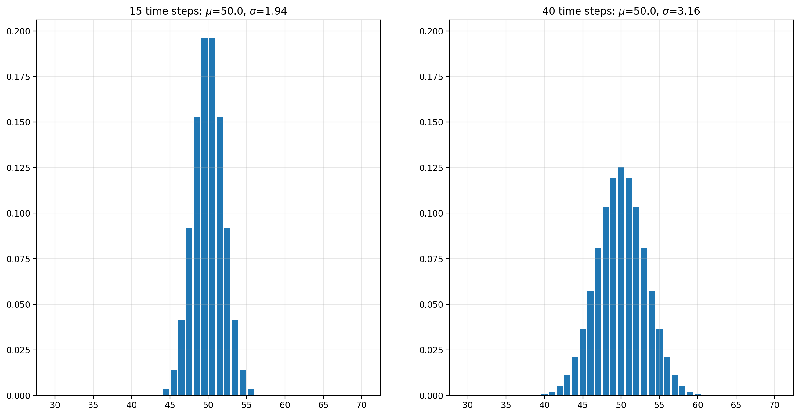
_images/2fb7f74c47c00806bfc781c4ce770214388cac7ef1fe6f50b1f1e6f7a3c5ab02.png

Exercise

What happens to this distribution when we change the probability, \(\pi\)?

paths

	n_up	n_down	Δs	paths	price	prob
node
0	0	15	-15	1	42.5	0.000031
1	1	14	-13	15	43.5	0.000458
2	2	13	-11	105	44.5	0.003204
3	3	12	-9	455	45.5	0.013885
4	4	11	-7	1365	46.5	0.041656
5	5	10	-5	3003	47.5	0.091644
6	6	9	-3	5005	48.5	0.152740
7	7	8	-1	6435	49.5	0.196381
8	8	7	1	6435	50.5	0.196381
9	9	6	3	5005	51.5	0.152740
10	10	5	5	3003	52.5	0.091644
11	11	4	7	1365	53.5	0.041656
12	12	3	9	455	54.5	0.013885
13	13	2	11	105	55.5	0.003204
14	14	1	13	15	56.5	0.000458
15	15	0	15	1	57.5	0.000031

There are \(2^n\) paths that a price can take over \(n\) time steps. For example, with \(n=25\) there are over 33.5 million paths.

n = 25
npaths = sum(binom(n, np.arange(n+1)))
print('{:,.0f}'.format(npaths))

33,554,432

While the code below isn’t a formal proof, it should convince you that

\[\sum_{k=0}^n \binom{n}{k} = 2^n.\]

for n in [5, 10, 25, 50, 100]:
    assert 2**n == sum(binom(n, np.arange(n+1)))

Or, we can ask Sympy to do the math for us:

import sympy as sp

n, k = sp.symbols('n k', integer=True, nonnegative=True)

expr = sp.summation(sp.binomial(n, k), (k, 0, n))

print("expr =", expr)

expr = 2**n

Exercise

Suppose we model each week of a year as being a single time step. How many possible paths are there to the terminal nodes?

Solution

With \(n=52\) there are over 4.5 quadrillion paths:

n = 52
print('{:,.0f}'.format(2**n))

4,503,599,627,370,496