
Principal Component Analysis#
import numpy as np
import pandas as pd
import matplotlib.pyplot as plt

import wrds
In the previous chapter, we decomposed stock returns using a factor model — the Fama-French 3-factor model. We regressed each stock’s excess return on the market, SMB, and HML factors, and showed that these three factors explain a substantial portion of the variation in individual stock returns.
But where did these factors come from? Fama and French chose them based on economic theory and empirical observation. What if instead of starting with a theory, we let the data tell us the most important sources of variation in stock returns?
This is exactly what Principal Component Analysis (PCA) does. PCA is a statistical technique that finds the directions of greatest variance in a dataset. Applied to stock returns, PCA will discover the common factors that drive returns — without any economic theory at all.
Dow Jones constituents#
As and example, we’ll begin by getting data for the stocks that make up the Dow Jones Industrial Average.
dow = pd.read_csv('https://raw.githubusercontent.com/stoffprof/qf_data/main/dow_current_components.csv')

dow
| company | ticker | permno | |
|---|---|---|---|
| 0 | 3M Company | MMM | 22592 |
| 1 | Amazon.com, Inc. | AMZN | 84788 |
| 2 | American Express Company | AXP | 59176 |
| 3 | Amgen Inc. | AMGN | 14008 |
| 4 | Apple Inc. | AAPL | 14593 |
| 5 | Caterpillar Inc. | CAT | 18542 |
| 6 | Cisco Systems, Inc. | CSCO | 76076 |
| 7 | Honeywell International Inc. | HON | 10145 |
| 8 | JPMorgan Chase & Co. | JPM | 47896 |
| 9 | Johnson & Johnson | JNJ | 22111 |
| 10 | Microsoft Corporation | MSFT | 10107 |
| 11 | Nike, Inc. | NKE | 57665 |
| 12 | Nvidia Corporation | NVDA | 86580 |
| 13 | Salesforce, Inc. | CRM | 90215 |
| 14 | The Boeing Company | BA | 19561 |
| 15 | The Coca-Cola Company | KO | 11308 |
| 16 | The Goldman Sachs Group, Inc. | GS | 86868 |
| 17 | The Home Depot, Inc. | HD | 66181 |
| 18 | The Procter & Gamble Company | PG | 18163 |
| 19 | The Sherwin-Williams Company | SHW | 36468 |
| 20 | The Travelers Companies, Inc. | TRV | 59459 |
| 21 | UnitedHealth Group Incorporated | UNH | 92655 |
| 22 | Verizon Communications Inc. | VZ | 65875 |
| 23 | Visa Inc. | V | 92611 |
| 24 | Walmart Inc. | WMT | 55976 |
| 25 | Merck & Co., Inc. | MRK | 22752 |
| 26 | The Walt Disney Company | DIS | 26403 |
| 27 | McDonald's Corporation | MCD | 43449 |
| 28 | Chevron Corporation | CVX | 14541 |
| 29 | International Business Machines Corporation | IBM | 12490 |
db = wrds.Connection()
Loading library list...
Done
sql = """
      SELECT permno, ticker, dlycaldt, dlyret
      FROM crsp.dsf_v2
      WHERE permno IN %(permnos)s
      AND dlycaldt >= '2020-01-01'
      """

params = {'permnos': tuple(dow['permno'].to_list())}

rets = db.raw_sql(sql, params=params, date_cols=['dlycaldt'])
rets
| permno | ticker | dlycaldt | dlyret | |
|---|---|---|---|---|
| 0 | 10107 | MSFT | 2020-01-02 | 0.018516 |
| 1 | 10107 | MSFT | 2020-01-03 | -0.012452 |
| 2 | 10107 | MSFT | 2020-01-06 | 0.002585 |
| 3 | 10107 | MSFT | 2020-01-07 | -0.009118 |
| 4 | 10107 | MSFT | 2020-01-08 | 0.015928 |
| ... | ... | ... | ... | ... |
| 45235 | 92655 | UNH | 2025-12-24 | 0.008559 |
| 45236 | 92655 | UNH | 2025-12-26 | 0.012974 |
| 45237 | 92655 | UNH | 2025-12-29 | -0.008709 |
| 45238 | 92655 | UNH | 2025-12-30 | 0.009789 |
| 45239 | 92655 | UNH | 2025-12-31 | -0.006172 |
45240 rows × 4 columns
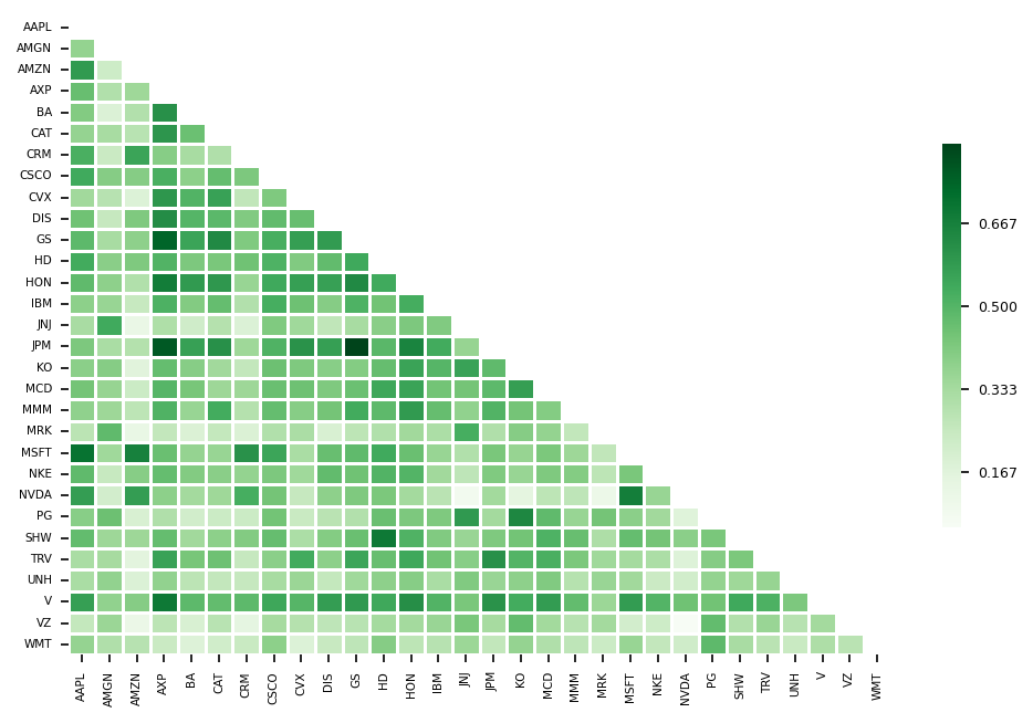
This dataframe is in a “long” format, with the data for each firm stacked one after another. In order to look at the correlations among firm returns, we need to reshape the data so each stock is in it’s own column.
rets = rets.pivot(index='dlycaldt', columns='ticker', values='dlyret').sort_index(axis=1)

rets
| ticker | AAPL | AMGN | AMZN | AXP | BA | CAT | CRM | CSCO | CVX | DIS | ... | MSFT | NKE | NVDA | PG | SHW | TRV | UNH | V | VZ | WMT |
|---|---|---|---|---|---|---|---|---|---|---|---|---|---|---|---|---|---|---|---|---|---|
| dlycaldt | |||||||||||||||||||||
| 2020-01-02 | 0.022816 | -0.004024 | 0.027151 | 0.014379 | 0.023207 | 0.019299 | 0.026746 | 0.016889 | 0.007634 | 0.024684 | ... | 0.018516 | 0.008785 | 0.019592 | -0.01193 | -0.020033 | 0.004089 | -0.005034 | 0.017137 | -0.0057 | 0.000841 |
| 2020-01-03 | -0.009722 | -0.006789 | -0.012139 | -0.009932 | -0.00168 | -0.013884 | -0.00491 | -0.016316 | -0.003459 | -0.011471 | ... | -0.012452 | -0.00274 | -0.016006 | -0.006726 | -0.012941 | -0.003563 | -0.01012 | -0.007953 | -0.010647 | -0.008828 |
| 2020-01-06 | 0.007968 | 0.007674 | 0.014886 | -0.004334 | 0.002945 | -0.000674 | 0.043811 | 0.003569 | -0.003388 | -0.005802 | ... | 0.002585 | -0.000883 | 0.004194 | 0.001387 | -0.001843 | 0.001095 | 0.006942 | -0.002162 | -0.002152 | -0.002036 |
| 2020-01-07 | -0.004703 | -0.009405 | 0.002092 | -0.005239 | 0.010607 | -0.013213 | 0.014702 | -0.006485 | -0.01277 | 0.000343 | ... | -0.009118 | -0.000491 | 0.012107 | -0.006191 | -0.005413 | -0.014653 | -0.006037 | -0.002643 | -0.011117 | -0.009265 |
| 2020-01-08 | 0.016086 | 0.000756 | -0.007809 | 0.01726 | -0.017523 | 0.008881 | 0.007557 | 0.000632 | -0.011423 | -0.002059 | ... | 0.015928 | -0.00226 | 0.001876 | 0.004263 | 0.015918 | 0.010728 | 0.021084 | 0.017118 | 0.001846 | -0.003432 |
| ... | ... | ... | ... | ... | ... | ... | ... | ... | ... | ... | ... | ... | ... | ... | ... | ... | ... | ... | ... | ... | ... |
| 2025-12-24 | 0.005324 | 0.007451 | 0.001034 | 0.002407 | 0.006041 | 0.002301 | 0.006947 | 0.0 | -0.000066 | 0.011129 | ... | 0.002403 | 0.04639 | -0.003171 | 0.009149 | 0.004012 | 0.004719 | 0.008559 | 0.00498 | 0.01002 | 0.006402 |
| 2025-12-26 | -0.001497 | -0.003084 | 0.000602 | -0.005377 | -0.007884 | -0.001302 | 0.003091 | 0.001794 | -0.003189 | -0.008036 | ... | -0.000635 | 0.0155 | 0.01018 | 0.00173 | 0.000277 | -0.005854 | 0.012974 | -0.000394 | 0.003968 | 0.001165 |
| 2025-12-29 | 0.001317 | -0.009912 | -0.001935 | -0.015037 | 0.003742 | -0.00753 | 0.000564 | -0.004734 | 0.006466 | 0.005548 | ... | -0.001251 | 0.004595 | -0.012124 | -0.001175 | -0.000645 | -0.00065 | -0.008709 | -0.001099 | 0.0 | 0.00707 |
| 2025-12-30 | -0.002484 | -0.002852 | 0.001982 | -0.005142 | 0.005754 | -0.002109 | -0.001164 | -0.004885 | 0.008742 | 0.005254 | ... | 0.00078 | -0.000327 | -0.003613 | -0.003597 | 0.00286 | 0.001541 | 0.009789 | -0.002792 | 0.005435 | -0.005421 |
| 2025-12-31 | -0.004468 | -0.004198 | -0.007354 | -0.009213 | -0.006316 | -0.007828 | -0.003798 | -0.004909 | 0.000657 | -0.008886 | ... | -0.007918 | 0.041183 | -0.005545 | -0.005137 | -0.006531 | -0.007935 | -0.006172 | -0.008229 | 0.000737 | -0.004557 |
1508 rows × 30 columns
rets.corr()
| ticker | AAPL | AMGN | AMZN | AXP | BA | CAT | CRM | CSCO | CVX | DIS | ... | MSFT | NKE | NVDA | PG | SHW | TRV | UNH | V | VZ | WMT |
|---|---|---|---|---|---|---|---|---|---|---|---|---|---|---|---|---|---|---|---|---|---|
| ticker | |||||||||||||||||||||
| AAPL | 1.000000 | 0.372698 | 0.588565 | 0.464588 | 0.408966 | 0.369408 | 0.521615 | 0.540079 | 0.344762 | 0.449628 | ... | 0.709334 | 0.479990 | 0.578697 | 0.397282 | 0.472431 | 0.323185 | 0.320916 | 0.572172 | 0.255233 | 0.370929 |
| AMGN | 0.372698 | 1.000000 | 0.227641 | 0.304566 | 0.182768 | 0.327351 | 0.242629 | 0.403563 | 0.288820 | 0.252920 | ... | 0.347816 | 0.251003 | 0.214736 | 0.453415 | 0.352975 | 0.330391 | 0.377750 | 0.380859 | 0.359040 | 0.306147 |
| AMZN | 0.588565 | 0.227641 | 1.000000 | 0.350820 | 0.302305 | 0.285735 | 0.556095 | 0.402166 | 0.182239 | 0.418601 | ... | 0.665179 | 0.400072 | 0.578519 | 0.195819 | 0.352554 | 0.160185 | 0.183208 | 0.403118 | 0.121580 | 0.290397 |
| AXP | 0.464588 | 0.304566 | 0.350820 | 1.000000 | 0.616399 | 0.601308 | 0.401060 | 0.520066 | 0.598165 | 0.627924 | ... | 0.461831 | 0.469285 | 0.388715 | 0.307739 | 0.470060 | 0.564530 | 0.376842 | 0.689667 | 0.277706 | 0.240530 |
| BA | 0.408966 | 0.182768 | 0.302305 | 0.616399 | 1.000000 | 0.458273 | 0.329436 | 0.387195 | 0.505067 | 0.499486 | ... | 0.371455 | 0.409898 | 0.336690 | 0.218302 | 0.344662 | 0.432992 | 0.276272 | 0.484157 | 0.196765 | 0.177394 |
| CAT | 0.369408 | 0.327351 | 0.285735 | 0.601308 | 0.458273 | 1.000000 | 0.307555 | 0.470481 | 0.565401 | 0.487352 | ... | 0.365237 | 0.395954 | 0.350437 | 0.235023 | 0.387264 | 0.450491 | 0.258833 | 0.473855 | 0.285614 | 0.219436 |
| CRM | 0.521615 | 0.242629 | 0.556095 | 0.401060 | 0.329436 | 0.307555 | 1.000000 | 0.420942 | 0.265028 | 0.411995 | ... | 0.613328 | 0.373062 | 0.525674 | 0.234544 | 0.408523 | 0.252194 | 0.254354 | 0.483644 | 0.149421 | 0.243560 |
| CSCO | 0.540079 | 0.403563 | 0.402166 | 0.520066 | 0.387195 | 0.470481 | 0.420942 | 1.000000 | 0.418337 | 0.474927 | ... | 0.552759 | 0.421750 | 0.439537 | 0.443482 | 0.465585 | 0.390867 | 0.327715 | 0.548290 | 0.332182 | 0.388439 |
| CVX | 0.344762 | 0.288820 | 0.182239 | 0.598165 | 0.505067 | 0.565401 | 0.265028 | 0.418337 | 1.000000 | 0.465362 | ... | 0.322090 | 0.347589 | 0.252549 | 0.243176 | 0.315675 | 0.534679 | 0.359316 | 0.497087 | 0.296481 | 0.180972 |
| DIS | 0.449628 | 0.252920 | 0.418601 | 0.627924 | 0.499486 | 0.487352 | 0.411995 | 0.474927 | 0.465362 | 1.000000 | ... | 0.463806 | 0.475274 | 0.386416 | 0.283895 | 0.405213 | 0.388714 | 0.255559 | 0.577465 | 0.272288 | 0.247206 |
| GS | 0.483475 | 0.328065 | 0.386454 | 0.746153 | 0.556916 | 0.637624 | 0.414591 | 0.524205 | 0.575054 | 0.585542 | ... | 0.479904 | 0.448737 | 0.419982 | 0.302804 | 0.460269 | 0.552762 | 0.347310 | 0.589768 | 0.285640 | 0.272102 |
| HD | 0.536499 | 0.393623 | 0.418300 | 0.507309 | 0.421740 | 0.429114 | 0.447851 | 0.511961 | 0.411454 | 0.476504 | ... | 0.539301 | 0.507317 | 0.425609 | 0.460134 | 0.689482 | 0.463651 | 0.386319 | 0.544729 | 0.334142 | 0.405170 |
| HON | 0.478002 | 0.386366 | 0.303614 | 0.676312 | 0.586627 | 0.596636 | 0.363728 | 0.542813 | 0.571305 | 0.569285 | ... | 0.462178 | 0.503209 | 0.338508 | 0.422328 | 0.507583 | 0.543798 | 0.399333 | 0.623669 | 0.337499 | 0.275358 |
| IBM | 0.388039 | 0.363489 | 0.251397 | 0.515687 | 0.410131 | 0.469301 | 0.302104 | 0.527384 | 0.452859 | 0.404337 | ... | 0.363539 | 0.343250 | 0.284737 | 0.419280 | 0.412361 | 0.446925 | 0.323580 | 0.507143 | 0.360402 | 0.289566 |
| JNJ | 0.325489 | 0.539199 | 0.125530 | 0.311145 | 0.223201 | 0.296031 | 0.183663 | 0.414222 | 0.345219 | 0.267851 | ... | 0.303010 | 0.270663 | 0.083326 | 0.591703 | 0.360348 | 0.397157 | 0.412243 | 0.427085 | 0.426305 | 0.354220 |
| JPM | 0.422049 | 0.321624 | 0.298973 | 0.776750 | 0.569423 | 0.618827 | 0.350898 | 0.508758 | 0.612632 | 0.571619 | ... | 0.427012 | 0.415975 | 0.341754 | 0.338611 | 0.417677 | 0.616895 | 0.362399 | 0.612432 | 0.330122 | 0.261934 |
| KO | 0.390138 | 0.404943 | 0.166679 | 0.469218 | 0.401141 | 0.344236 | 0.259800 | 0.456227 | 0.420166 | 0.397577 | ... | 0.366908 | 0.365330 | 0.155023 | 0.646636 | 0.443732 | 0.501940 | 0.384966 | 0.533396 | 0.472627 | 0.371085 |
| MCD | 0.440202 | 0.367915 | 0.234836 | 0.496450 | 0.432544 | 0.353689 | 0.353726 | 0.461637 | 0.452902 | 0.420084 | ... | 0.426040 | 0.419180 | 0.275184 | 0.479922 | 0.511896 | 0.519601 | 0.413106 | 0.581576 | 0.339063 | 0.306192 |
| MMM | 0.382275 | 0.351190 | 0.274413 | 0.509391 | 0.364273 | 0.532627 | 0.294764 | 0.470543 | 0.400574 | 0.440202 | ... | 0.351507 | 0.407161 | 0.271369 | 0.364037 | 0.464411 | 0.423952 | 0.291942 | 0.471409 | 0.289976 | 0.269999 |
| MRK | 0.280452 | 0.477731 | 0.130039 | 0.260542 | 0.186023 | 0.256410 | 0.186759 | 0.302858 | 0.318486 | 0.196915 | ... | 0.266531 | 0.274815 | 0.118893 | 0.440882 | 0.313612 | 0.345820 | 0.360194 | 0.355980 | 0.338002 | 0.234759 |
| MSFT | 0.709334 | 0.347816 | 0.665179 | 0.461831 | 0.371455 | 0.365237 | 0.613328 | 0.552759 | 0.322090 | 0.463806 | ... | 1.000000 | 0.428815 | 0.675745 | 0.390881 | 0.469396 | 0.334754 | 0.341997 | 0.579932 | 0.212997 | 0.364336 |
| NKE | 0.479990 | 0.251003 | 0.400072 | 0.469285 | 0.409898 | 0.395954 | 0.373062 | 0.421750 | 0.347589 | 0.475274 | ... | 0.428815 | 1.000000 | 0.364749 | 0.342250 | 0.438689 | 0.315364 | 0.237059 | 0.501999 | 0.227829 | 0.258685 |
| NVDA | 0.578697 | 0.214736 | 0.578519 | 0.388715 | 0.336690 | 0.350437 | 0.525674 | 0.439537 | 0.252549 | 0.386416 | ... | 0.675745 | 0.364749 | 1.000000 | 0.170916 | 0.391632 | 0.178149 | 0.217265 | 0.448263 | 0.056020 | 0.223718 |
| PG | 0.397282 | 0.453415 | 0.195819 | 0.307739 | 0.218302 | 0.235023 | 0.234544 | 0.443482 | 0.243176 | 0.283895 | ... | 0.390881 | 0.342250 | 0.170916 | 1.000000 | 0.427550 | 0.403076 | 0.373357 | 0.446810 | 0.471544 | 0.480696 |
| SHW | 0.472431 | 0.352975 | 0.352554 | 0.470060 | 0.344662 | 0.387264 | 0.408523 | 0.465585 | 0.315675 | 0.405213 | ... | 0.469396 | 0.438689 | 0.391632 | 0.427550 | 1.000000 | 0.425959 | 0.349141 | 0.543030 | 0.300739 | 0.325499 |
| TRV | 0.323185 | 0.330391 | 0.160185 | 0.564530 | 0.432992 | 0.450491 | 0.252194 | 0.390867 | 0.534679 | 0.388714 | ... | 0.334754 | 0.315364 | 0.178149 | 0.403076 | 0.425959 | 1.000000 | 0.366954 | 0.515575 | 0.360751 | 0.283174 |
| UNH | 0.320916 | 0.377750 | 0.183208 | 0.376842 | 0.276272 | 0.258833 | 0.254354 | 0.327715 | 0.359316 | 0.255559 | ... | 0.341997 | 0.237059 | 0.217265 | 0.373357 | 0.349141 | 0.366954 | 1.000000 | 0.422002 | 0.290063 | 0.244062 |
| V | 0.572172 | 0.380859 | 0.403118 | 0.689667 | 0.484157 | 0.473855 | 0.483644 | 0.548290 | 0.497087 | 0.577465 | ... | 0.579932 | 0.501999 | 0.448263 | 0.446810 | 0.543030 | 0.515575 | 0.422002 | 1.000000 | 0.337077 | 0.313942 |
| VZ | 0.255233 | 0.359040 | 0.121580 | 0.277706 | 0.196765 | 0.285614 | 0.149421 | 0.332182 | 0.296481 | 0.272288 | ... | 0.212997 | 0.227829 | 0.056020 | 0.471544 | 0.300739 | 0.360751 | 0.290063 | 0.337077 | 1.000000 | 0.282519 |
| WMT | 0.370929 | 0.306147 | 0.290397 | 0.240530 | 0.177394 | 0.219436 | 0.243560 | 0.388439 | 0.180972 | 0.247206 | ... | 0.364336 | 0.258685 | 0.223718 | 0.480696 | 0.325499 | 0.283174 | 0.244062 | 0.313942 | 0.282519 | 1.000000 |
30 rows × 30 columns
Eigenvalues and Eigenvectors#
For an \(N\times N\) matrix \(A\), a scalar \(\lambda\) and non-zero vector \(\mathbf{v}\) satisfying
are called an eigenvalue and eigenvector of \(A\), respectively.
We want to find \(\lambda\) and non-zero \(\mathbf{v}\) such that \(A \mathbf{v} = \lambda \mathbf{v}\). Rearranging:
This has a non-zero solution \(\mathbf{v}\) if and only if the matrix \((A - \lambda I)\) is singular — that is, it cannot be inverted. A matrix is singular if and only if its determinant is zero, so we require:
This is the characteristic equation. Any \(\lambda\) satisfying it is an eigenvalue, and the corresponding eigenvector \(\mathbf{v}\) is then found by solving \((A - \lambda I)\mathbf{v} = \mathbf{0}\) directly.
Since the characteristic equation actually defines a system of \(N\) equations, there are \(N\) solutions, each of which gives an eigenvalue and corresponding eigenvector.
Having found the eigenvalues and eigenvectors, we can collect them into two matrices:
\(\boldsymbol{\Lambda}\) is a diagonal matrix of eigenvalues \(\lambda_1 \geq \lambda_2 \geq \cdots \geq \lambda_N\); and
\(\mathbf{V}\) is a matrix whose columns are the corresponding eigenvectors.
This allows us to decompose the matrix \(A\) as follows:
In other words, the matrix \(A\) is completely characterized by its eigenvalues and eigenvectors. This is called the eigendecomposition.
Calculation example#
Let
Begin by finding the characteristic equation:
Next we solve the equation to find the eigenvalues. There are two in this case, because \(A\) is \(2\times 2\).
Note that \(\lambda_1 + \lambda_2 = 7 = \text{tr}(A)\).
Next, we solve for the eigenvectors. For each \(\lambda_i\), solve \((A - \lambda_i I)\mathbf{v} = \mathbf{0}\). The first row gives:
For \(\lambda_1 \approx 5.561\):
Setting \(v_1 = 1\), the unnormalized vector is \(\begin{bmatrix} 1 \\ 0.781 \end{bmatrix}\), with length \(\sqrt{1 + 0.781^2} = \sqrt{1.610} \approx 1.269\). Dividing through by this, we get
For \(\lambda_2 \approx 1.439\):
Setting \(v_1 = 1\), the unnormalized vector is \(\begin{bmatrix} 1 \\ -1.281 \end{bmatrix}\), with length \(\sqrt{1 + 1.281^2} = \sqrt{2.641} \approx 1.625\). Again, dividing by this, we find
We can now use
to confirm the decomposition
V = np.array([[0.788, 0.615],
              [0.615, -0.788]])

L = np.array([[5.561, 0],
              [0, 1.439]])

V @ L @ V.T
array([[3.99733536, 1.99760364],
       [1.99760364, 2.99684764]])
There’s some small rounding error here, but this is very close to the original \(A\) matrix.
What is PCA?#
Suppose we have a matrix of returns \(\mathbf{R}\) with \(T\) rows (time periods) and \(N\) columns (stocks). The covariance matrix of returns is the \(N \times N\) matrix
PCA is the eigendecomposition of the covariance matrix. Each eigenvector (also called the loadings or weights) defines a principal component — a linear combination of the original variables. In the case of stock returns, each principal component is therefore a portfolio return, where the eigenvector elements are the portfolio weights. The corresponding eigenvalue tells us how much variance that portfolio captures.
Geometrically, since \(\mathbf{v}\) is a direction that the matrix only stretches (by factor \(\lambda\)) rather than rotates, the eigenvectors of a covariance matrix identify the directions of greatest spread in the data, and the corresponding eigenvalues measure the amount of variance along each of those directions. For a symmetric matrix like \(\Sigma\), eigenvectors corresponding to distinct eigenvalues are always orthogonal, meaning the principal directions are perpendicular to one another. This orthogonality is what makes PCA a rotation of the original coordinate axes rather than an arbitrary transformation: the data is re-expressed in a new basis of mutually perpendicular directions, ordered from most to least variance.
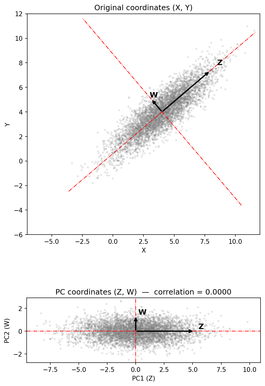
The scatter plot below shows 5,000 draws from a bivariate normal distribution with positive covariance between X and Y. The two arrows are the eigenvectors of the covariance matrix, and their lengths are proportional to \(\sqrt{\lambda_i}\) — the standard deviation along each principal axis.
The longer axis Z points in the direction of greatest variance in the data: it aligns roughly with the major axis of the elliptical cloud. The shorter axis W is perpendicular to Z and captures the remaining variance. Together, Z and W form a new coordinate system that is rotated relative to the original X-Y axes.
The dashed lines extend each eigenvector direction across the full plot, making it clear that PCA is identifying the natural axes of the data rather than the arbitrary axes we happened to measure it on.
If we project each data point onto Z and W instead of X and Y, the resulting coordinates will be uncorrelated, as shown in the second figure. Projection here simply means measuring how far each point lies along each axis — the same way an X coordinate measures how far a point lies along the horizontal axis, but now measured along the tilted PC axes instead. This is the core operation of PCA.
Key fact
PCA finds orthogonal (uncorrelated) linear combinations of the original variables that capture the maximum amount of variance. The fraction of total variance explained by the \(k\)-th principal component is
The first principal component captures the most variance, the second captures the most of what’s left, and so on.
The sum of the eigenvalues equals the sum of variances, which equals the trace of the covariance matrix:
Example: The 2×2 Case#
We can gain some intuition by considering the simplest case of two stocks. Let the variance-covariance matrix be:
Step 1: Find the Characteristic Equation
Step 2: Solve for the eigenvalues
Applying the quadratic formula, with discriminant:
gives:
Step 3: Find the eigenvectors
For each eigenvalue, solve \((\Sigma - \lambda I)\mathbf{v} = \mathbf{0}\). The first row gives:
so the eigenvector corresponding to each \(\lambda\) is proportional to:
Substituting \(\lambda_1\) and \(\lambda_2\) gives two orthogonal eigenvectors, which can be normalized by dividing by their lengths:
There are two special cases worth considering:
Special Case #1: Equal Variances \((\sigma_1^2 = \sigma_2^2 = \sigma^2)\)
Substituting into the eigenvalues, the \((\sigma_1^2 - \sigma_2^2)^2\) term vanishes:
The eigenvalues are symmetric around \(\sigma^2\), and total variance \(\lambda_1 + \lambda_2 = 2\sigma^2\) is preserved. As \(\rho \to 1\), all variance concentrates in PC1 and \(\lambda_2 \to 0\) — the two variables become a single factor. As \(\rho \to 0\), both eigenvalues equal \(\sigma^2\) and the two PCs are equivalent.
For the eigenvectors, substituting \(\sigma_1^2 = \sigma_2^2 = \sigma^2\) into the general formula \(\mathbf{v} \propto \begin{bmatrix} 2\rho\sigma_1\sigma_2 \\ \sigma_2^2 - \sigma_1^2 \pm \sqrt{\Delta} \end{bmatrix}\), the \((\sigma_2^2 - \sigma_1^2)\) terms vanish and \(\sqrt{\Delta} = 2\rho\sigma^2\):
The principal axes are the 45° diagonals, regardless of \(\rho\) (as long as \(\rho \neq 0\)). PC1 points in the direction of the sum \(X_1 + X_2\) — the direction along which the two variables move together — and PC2 points in the direction of the difference \(X_1 - X_2\), along which they move against each other.
This has a natural financial interpretation: if two assets have equal variance, the first principal component is essentially the average return (long both, like a portfolio) and the second is the spread (long one, short the other, like a pairs trade). The more correlated the assets, the more variance is concentrated in the sum direction and the less in the spread direction.
Special Case #2: \(\rho = 0\)
When the variables are uncorrelated the matrix is already diagonal, and the eigenvalues and eigenvectors reduce to:
The principal axes coincide with the original coordinate axes, as expected.
As an example, let’s take only the first three stocks in our data, and calculate the eigenvector decomposition from their covariances.
cov = (rets.iloc[:, :3] * 100).cov()

cov
| ticker | AAPL | AMGN | AMZN |
|---|---|---|---|
| ticker | |||
| AAPL | 4.015538 | 1.242392 | 2.652895 |
| AMGN | 1.242392 | 2.767313 | 0.851792 |
| AMZN | 2.652895 | 0.851792 | 5.059491 |
eigvals, eigvecs = np.linalg.eigh(cov)

# need to sort the eigenvalues and eigenvectors in descending order
idx = np.argsort(eigvals)[::-1]   # descending order
eigvals = eigvals[idx]
eigvecs = eigvecs[:, idx]
eigvals
array([7.67092163, 2.56083097, 1.6105894 ])
np.diag(eigvals)
array([[7.67092163, 0.        , 0.        ],
       [0.        , 2.56083097, 0.        ],
       [0.        , 0.        , 1.6105894 ]])
eigvecs
array([[-0.6245524 , -0.20777194, -0.75283804],
       [-0.28457398, -0.83714691,  0.46712172],
       [-0.72729083,  0.50598011,  0.46371562]])
Note that we can recover the covariance matrix frmo the eigenvectors and eigenvalues using the equation above.
eigvecs @ np.diag(eigvals) @ eigvecs.T
array([[4.01553827, 1.24239198, 2.65289473],
       [1.24239198, 2.76731284, 0.8517921 ],
       [2.65289473, 0.8517921 , 5.05949088]])
As expected, the sum of the eigenvalues equals the sum of the variances:
sum(eigvals)
11.842341993240536
np.diag(cov).sum()
11.84234199324054
The three eigenvalues and corresponding proportion of variance explained by each principal component are:
for i, eigval in enumerate(eigvals):
    print(f"Eigenvalue {i+1}: {eigval:.4f} ({eigval / sum(eigvals) * 100:.1f}%)")
Eigenvalue 1: 7.6709 (64.8%)
Eigenvalue 2: 2.5608 (21.6%)
Eigenvalue 3: 1.6106 (13.6%)
Fitting PCA#
Now we can fit PCA to all 30 stocks in the Dow index.
pca = PCA()
pca.fit(rets)
PCA()In a Jupyter environment, please rerun this cell to show the HTML representation or trust the notebook.
On GitHub, the HTML representation is unable to render, please try loading this page with nbviewer.org.
Parameters
| n_components | None | |
| copy | True | |
| whiten | False | |
| svd_solver | 'auto' | |
| tol | 0.0 | |
| iterated_power | 'auto' | |
| n_oversamples | 10 | |
| power_iteration_normalizer | 'auto' | |
| random_state | None |
print(f'Number of components: {pca.n_components_}')
print(f'Variance explained by first PC: {pca.explained_variance_ratio_[0]:.1%}')
print(f'Variance explained by first 3 PCs: {pca.explained_variance_ratio_[:3].sum():.1%}')
print(f'Variance explained by first 10 PCs: {pca.explained_variance_ratio_[:10].sum():.1%}')
Number of components: 30
Variance explained by first PC: 43.8%
Variance explained by first 3 PCs: 60.2%
Variance explained by first 10 PCs: 79.3%
Scree plot#
A scree plot shows the fraction of variance explained by each principal component. The name comes from the geological term for the pile of rocks at the base of a cliff — the plot looks like a steep cliff followed by a flat pile of rubble.
K = 10  # show first K components

fig, ax = plt.subplots(figsize=(6, 3))

# Bar chart of individual explained variance
ax.bar(range(1, K+1), pca.explained_variance_ratio_[:K],
       color='steelblue', edgecolor='k', alpha=0.7, label='Individual')

# Line plot of cumulative explained variance
ax2 = ax.twinx()
ax2.plot(range(1, K+1), np.cumsum(pca.explained_variance_ratio_[:K]),
         'o-', color='darkred', lw=2, ms=5, label='Cumulative')

ax.set_xlabel('Principal Component')
ax.set_ylabel('Fraction of Variance Explained')
ax2.set_ylabel('Cumulative Variance Explained')
ax.set_title('Scree Plot')
ax.set_xticks(range(1, K+1))

# Combine legends
lines1, labels1 = ax.get_legend_handles_labels()
lines2, labels2 = ax2.get_legend_handles_labels()
ax.legend(lines1 + lines2, labels1 + labels2, loc='center right')

ax.grid(alpha=0.3, axis='y')

plt.show()
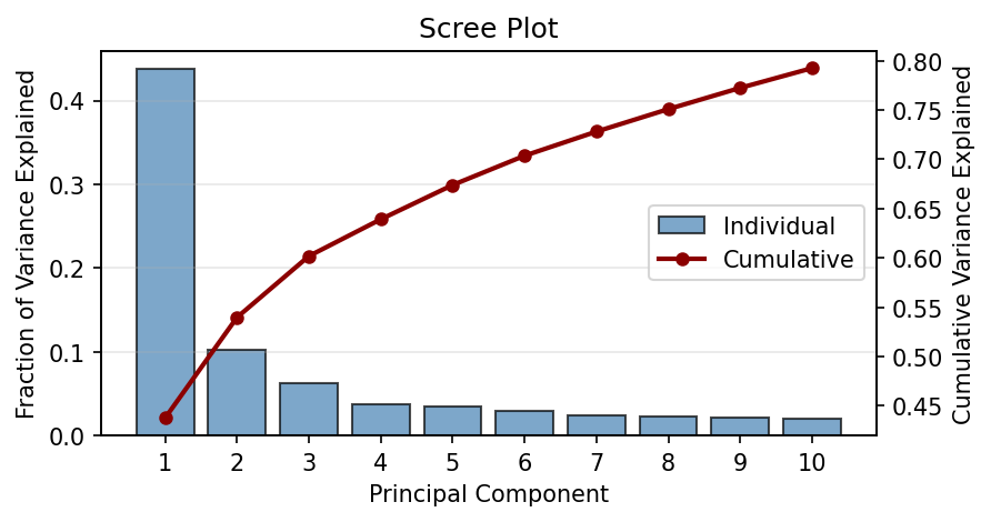
The first principal component dominates — it explains far more variance than any other single component. This is a well-known feature of stock returns: stocks tend to move together, driven by a single common “market” factor.
Interpreting principal components#
Each principal component is defined by a vector of loadings — one weight for each stock. Let’s look at the loadings of the first three principal components.
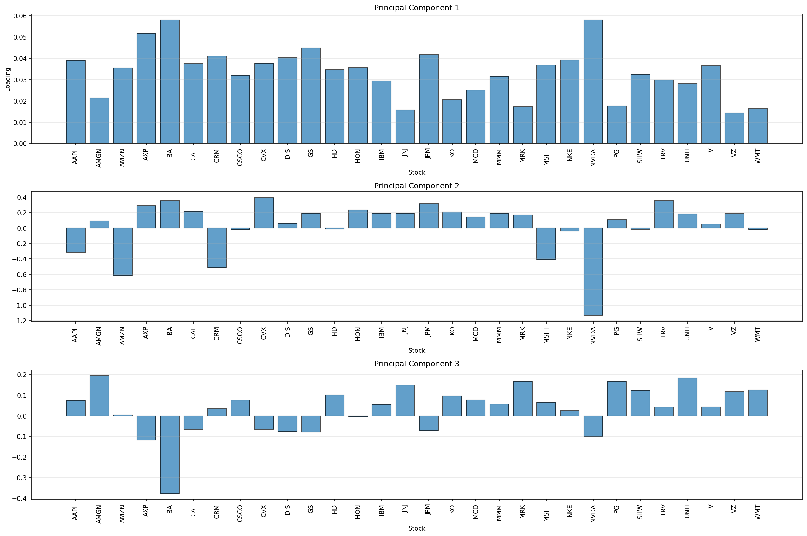
The first principal component has positive weight on all stocks, and the weights are fairly close to 0.03, which corresponds to an equal weight on all stocks in the index. In other words, PC1 corresponds pretty closely to the market portfolio. We can see this by looking at the correlations among an equal-weighted Dow portfolio, the Fama–French market portfolio, and PC1.
# 1) Equal-weighted portfolio return across the 30 Dow stocks
ew_port = rets.mean(axis=1)

# 2) Market return from Fama-French daily factors
ff = db.get_table('ff', 'factors_daily')
ff['date'] = pd.to_datetime(ff['date'])
ff = ff.set_index('date').sort_index()
mkt = ff['mktrf'] + ff['rf']

# 3) First principal-component score time series
pc1 = pd.Series(pca.transform(rets)[:, 0], index=rets.index, name='pc1')

# Align dates and compute pairwise correlations
corr_df = pd.concat([
    ew_port.rename('ew_port'),
    mkt.rename('mkt'),
    pc1
], axis=1).dropna()

corr_df.corr()
| ew_port | mkt | pc1 | |
|---|---|---|---|
| ew_port | 1.000000 | 0.953132 | 0.992252 |
| mkt | 0.953132 | 1.000000 | 0.964445 |
| pc1 | 0.992252 | 0.964445 | 1.000000 |
PC1 maximizes average \(R^2\)#
We’ve seen that PC1 looks a lot like the market — it has positive weight on every stock and explains the largest share of total variance. But we can make a stronger claim: PC1 is the single factor that best explains individual stock returns, in the sense of maximizing the average \(R^2\) across all stocks.
To see this, consider forming a candidate factor as a portfolio return:
where \(\mathbf{w}\) is some weight vector. For each stock \(i\), regress its return on the factor:
and record \(R^2_i\). Then compute the average across all 30 stocks:
The claim is: the weight vector \(\mathbf{w}\) that maximizes \(\bar{R}^2\) is precisely the first eigenvector.
We can verify this numerically. Below, we try 100,000 random weight vectors and compute \(\bar{R}^2\) for each. We then compare the best random vector to the first eigenvector from PCA.
def r2s_vectorized(R, f):
    '''
    Compute R^2 between each column of R and factor f.

    Parameters
    ----------
    R : array (T, N)
        Matrix of returns (T time periods, N assets)
    f : array (T,)
        Factor

    Returns
    -------
    r2s : array (N,)
        R^2 for regression of each column of R on f with intercept
    '''

    R = np.asarray(R)
    f = np.asarray(f)

    # Demean (equivalent to including intercept)
    Rc = R - R.mean(axis=0)
    fc = f - f.mean()

    # Covariance with factor
    cov = fc @ Rc

    # Variances
    var_f = fc @ fc
    var_R = np.sum(Rc**2, axis=0)

    # Correlation
    corr = cov / np.sqrt(var_f * var_R)

    return corr**2

def avg_r2(w, R):
    """Average R² from regressing each column of R on the factor w'R."""
    f = R @ w
    r2s = r2s_vectorized(R, f)
    return r2s.mean()


R = rets.to_numpy(dtype=float)
N = R.shape[1]

# --- Random search over 100,000 weight vectors ---
n_trials = 100_000
rng_search = np.random.default_rng(42)
best_r2_random = 0
best_w_random = None

for _ in range(n_trials):
    w = rng_search.normal(size=N)
    w = w / np.linalg.norm(w)   # normalize so weights sum to one
    r2 = avg_r2(w, R)
    if r2 > best_r2_random:
        best_r2_random = r2
        best_w_random = w

# --- First eigenvector from PCA ---
w_pc1 = pca.components_[0]
r2_pc1 = avg_r2(w_pc1, R)

print(f'Average R² using PC1 weights:           {r2_pc1:.6f}')
print(f'Best average R² from 100k random tries: {best_r2_random:.6f}')
Average R² using PC1 weights:           0.415639
Best average R² from 100k random tries: 0.410664
No random weight vector can beat PC1. This is not a coincidence — it is a mathematical property of the eigendecomposition. The first eigenvector of the covariance matrix defines the direction that maximizes the variance of the projected data, and maximizing the variance of a single factor is equivalent to maximizing the average \(R^2\) of individual regressions on that factor.
Interestingly, the random weights that come closest to explaining the most variation are nothing like the weights in PC1:
best_w_random
array([-0.12656536, -0.0178549 , -0.02130421, -0.09306356, -0.12076946,
       -0.13255932,  0.03796464, -0.22180042,  0.02787833, -0.10674491,
       -0.08927331, -0.26148374, -0.07184436, -0.1783589 ,  0.15739297,
       -0.30351353, -0.19744539, -0.06131585, -0.16368019, -0.44736973,
       -0.21245458, -0.07185023,  0.0275325 , -0.50145917, -0.08734835,
        0.03076371,  0.03924356,  0.05684753, -0.22145143, -0.12161234])
w_pc1
array([0.20253139, 0.11101268, 0.18420322, 0.26813552, 0.3009445 ,
       0.19434087, 0.21281547, 0.16601456, 0.19503764, 0.20906604,
       0.2318724 , 0.17974964, 0.18446533, 0.15243533, 0.08168023,
       0.21578408, 0.10660011, 0.12974605, 0.16362666, 0.0893042 ,
       0.19075013, 0.20321203, 0.30073486, 0.09092254, 0.16866732,
       0.15474742, 0.1457521 , 0.18887908, 0.07421308, 0.08463696])
def angle_between(u, v):
    cos_theta = np.dot(u, v) / (np.linalg.norm(u) * np.linalg.norm(v))
    return np.arccos(cos_theta)  # radians

angle_rad = angle_between(best_w_random, w_pc1)
angle_deg = np.degrees(angle_rad)

print(f'Angle between best random weights and PC1: {angle_deg:.2f} degrees')
Angle between best random weights and PC1: 122.24 degrees
Now suppose we want to find the best second factor. We already know PC1 is the optimal single factor. The natural next question is: keeping PC1 fixed, what additional factor \(g_t = \mathbf{w}'\mathbf{r}_t\) maximizes the average \(R^2\) from a two-factor regression?
In other words, we want the second factor that explains the most of what PC1 leaves unexplained.
By appealing to something called the Frisch-Waugh theorem, we know that the \(R^2\) improvement from adding \(g_t\) to a regression that already includes \(f_t\) is the same as the \(R^2\) from regressing the residuals from that regression on \(g_t\). So we can implement this in two steps: first regress each stock on PC1 and collect the residuals \(\hat{\varepsilon}_{i,t}\), then search for the weight vector \(\mathbf{w}\) that maximizes \(\bar{R}^2\) when we regress each stock’s residuals on \(g_t = \mathbf{w}'\hat{\boldsymbol{\varepsilon}}_t\). The claim is that this optimal \(\mathbf{w}\) is the second eigenvector.
# Step 1: regress each stock on PC1 and collect residuals
f1 = R @ w_pc1
fc1 = f1 - f1.mean()
betas = (fc1 @ (R - R.mean(axis=0))) / (fc1 @ fc1)
resids = R - R.mean(axis=0) - np.outer(fc1, betas)   # (T, N)

# Step 2: search over random weight vectors applied to the residuals
best_r2_random2 = 0
best_w_random2 = None
rng_search2 = np.random.default_rng(123)

for _ in range(n_trials):
    w = rng_search2.normal(size=N)
    w = w / np.linalg.norm(w)
    r2 = avg_r2(w, resids)
    if r2 > best_r2_random2:
        best_r2_random2 = r2
        best_w_random2 = w

# Step 3: compare to the second eigenvector
w_pc2 = pca.components_[1]
r2_pc2 = avg_r2(w_pc2, resids)

print(f'Average R² of residuals using PC2 weights:  {r2_pc2:.6f}')
print(f'Best average R² from 100k random tries:     {best_r2_random2:.6f}')
Average R² of residuals using PC2 weights:  0.132291
Best average R² from 100k random tries:     0.125119
Finally, as expected, the angle between PC1 and PC2 confirms that they are orthogonal.
angle_rad = angle_between(pca.components_[0], pca.components_[1])
angle_deg = np.degrees(angle_rad)

print(f'Angle between PC1 and PC2: {angle_deg:.2f} degrees')
Angle between PC1 and PC2: 90.00 degrees
Variance decomposition#
How does PCA’s variance decomposition compare to the factor model approach from the previous chapter? In the Fama-French 3-factor model, the \(R^2\) tells us how much of a stock’s return variance is explained by the three factors. Here, we can ask: how many principal components do we need to explain a comparable fraction of variance?
cumvar = np.cumsum(pca.explained_variance_ratio_)

# Find how many PCs needed for various thresholds
for threshold in [0.25, 0.50, 0.75, 0.90]:
    n_pcs = np.argmax(cumvar >= threshold) + 1
    print(f'{threshold:.0%} of variance explained by {n_pcs} principal components')
25% of variance explained by 1 principal components
50% of variance explained by 2 principal components
75% of variance explained by 8 principal components
90% of variance explained by 18 principal components
Exercise
In the previous chapter, the average \(R^2\) from 3-factor regressions was roughly 0.15–0.35 depending on the stock. How does this compare to the fraction of total variance explained by the first 3 principal components? Why might these numbers differ?
Hint: Think about what “variance explained” means in each context. The factor model’s \(R^2\) is computed stock-by-stock, while PCA’s explained variance ratio is computed across all stocks simultaneously.
Solution
The \(R^2\) from a factor regression tells us what fraction of a single stock’s variance is explained by the factors. PCA’s explained variance ratio tells us what fraction of the total variance across all stocks is explained by each component.
These are different quantities. PCA’s first 3 components may explain, say, 25% of the total variance, but this is an average across all stocks. Some stocks (those with high factor loadings) will have much more of their variance explained, while others will have less.
Additionally, PCA chooses components to maximize total explained variance, while the Fama-French factors were chosen based on economic theory. The Fama-French factors may do better at explaining certain stocks’ returns even if they explain less of the total cross-sectional variance.