%load_ext autoreload
%autoreload 2
from helper_functions import display_matrix

Efficient portfolios

Suppose we wish to find

\[\begin{equation*} \begin{aligned} \min_{\omega} \quad & \boldsymbol{\omega}'\boldsymbol{\Sigma}\boldsymbol{\omega} \\ \textrm{subject to} \quad & \boldsymbol{\omega}'\mathbf{1} = 1. \end{aligned} \end{equation*}\]

Here, \(\mathbf{1} = (1, \ldots, 1)'\) is an \(N\)-vector of ones. We’ll also define \(\boldsymbol{\mu} = (\mu_1, \cdots, \mu_N)'\) to be the vector of expected returns for the assets. I am following the convention that boldface indicates a vector or matrix, while scalars are in regular font.

For reasons that will soon become clear, let’s first define the following scalars:

\[\begin{align*} A&:=\boldsymbol{\mu}'\boldsymbol{\Sigma}^{-1} \boldsymbol{\mu}, \\ B&:=\boldsymbol{\mu}'\boldsymbol{\Sigma}^{-1} \mathbf{1}, \\ C&:=\mathbf{1}'\boldsymbol{\Sigma}^{-1} \mathbf{1}. \end{align*}\]

Each of these is the product of a \(1\times N\) vector, an \(N\times N\) matrix, and an \(N\times 1\) vector, so the result has dimension \(1\times 1\): that is, just a scalar. Note that since these are scalars, \(B'=B\), so \(\mathbf{1}'\boldsymbol{\Sigma}^{-1}\boldsymbol{\mu} = \boldsymbol{\mu}'\boldsymbol{\Sigma}^{-1} \mathbf{1}.\)

Notice also that \(C\) is simply the sum of all of the elements of \(\bsi\).

This is a constrained optimization problem that can be solved using the method of Lagrange multipliers. The solution is

\[\boldsymbol{\omega}_{\text{GMV}} = \frac{1}{C} \boldsymbol{\Sigma}^{-1} \mathbf{1}.\]

Extra credit

To solve the problem, we write the Lagrangian

\[\mathcal{L} = \boldsymbol{\omega}' \boldsymbol{\Sigma} \boldsymbol{\omega} - 2\lambda (\boldsymbol{\omega}' \mathbf{1} - 1)\]

where \(\lambda\) is the Lagrange multiplier. Then, we set the derivative equal to zero and solve for the optimal weights:

\[\frac{\partial \mathcal{L}}{\partial \boldsymbol{\omega}} = 2\boldsymbol{\Sigma} \boldsymbol{\omega} - 2\lambda \mathbf{1} = 0\]

\[\begin{align*} \Rightarrow \boldsymbol{\Sigma} \boldsymbol{\omega} &= \lambda \mathbf{1} \\ \Rightarrow \boldsymbol{\omega} &= \lambda \boldsymbol{\Sigma}^{-1} \mathbf{1}. \end{align*}\]

We can find the value of \(\lambda\) by substituting this back into the constraint:

\[\begin{align*} \left(\lambda \boldsymbol{\Sigma}^{-1} \mathbf{1}\right)' \mathbf{1} &= 1 \\ \Rightarrow \lambda \mathbf{1}' \boldsymbol{\Sigma}^{-1} \mathbf{1} &= 1 \\ \Rightarrow \lambda C &= 1 \\ \end{align*}\]

Therefore, \(\lambda = \frac{1}{C},\) which gives the expected result:

\[\boldsymbol{\omega}_{\text{GMV}} = \frac{1}{C} \boldsymbol{\Sigma}^{-1} \mathbf{1}. \quad\blacksquare\]

These weights generate the portfolio with the minimum possible variance. The variance of this portfolio is

\[\begin{align*} \var(R_{\text{GMV}}) &= \boldsymbol{\omega}_{\text{GMV}}' \; \bs \; \boldsymbol{\omega}_{\text{GMV}} \\ &= \left(\frac{1}{C} \boldsymbol{\Sigma}^{-1} \mathbf{1}\right)' \boldsymbol{\Sigma} \left(\frac{1}{C} \boldsymbol{\Sigma}^{-1} \mathbf{1}\right) \\ &= \frac{1}{C^2} \mathbf{1}' \boldsymbol{\Sigma}^{-1} \boldsymbol{\Sigma} \boldsymbol{\Sigma}^{-1} \mathbf{1} \\ &= \frac{1}{C^2} \mathbf{1}' \boldsymbol{\Sigma}^{-1} \mathbf{1} \\ &= \frac{1}{C}. \end{align*}\]

To develop some intuition for what these values mean, let’s consider the simplest case of two assets.

\[\begin{split}\bs = \begin{bmatrix} \sigma_1^2 & \sigma_{12} \\ \sigma_{12} & \sigma_2^2 \end{bmatrix}, \qquad \bsi = \frac{1}{\Delta} \begin{bmatrix} \sigma_2^2 & -\sigma_{12} \\ -\sigma_{12} & \sigma_1^2 \end{bmatrix}, \end{split}\]

where \(\Delta = \sigma_1^2\sigma_2^2 - \sigma_{12}^2\) is the determinant of \(\bs\).

Then

\[C = \mathbf{1}' \Sigma^{-1} \mathbf{1} = \frac{1}{\Delta}(\sigma_1^2 - 2\sigma_{12} + \sigma_2^2).\]

So the final expression is:

\[C = \dfrac{\sigma_1^2 - 2\sigma_{12} + \sigma_2^2}{\sigma_1^2\sigma_2^2 - \sigma_{12}^2}\]

The weights on the two assets in the GMV are therefore:

\[\begin{split} \begin{aligned} \omega_1^{\text{GMV}} &= \frac{\sigma_2^2 - \sigma_{12}}{\sigma_1^2 - 2\sigma_{12} + \sigma_2^2}, \\[12pt] \omega_2^{\text{GMV}} &= \frac{\sigma_1^2 - \sigma_{12}}{\sigma_1^2 - 2\sigma_{12} + \sigma_2^2}. \end{aligned} \end{split}\]

You shouldn’t be surprised that these exactly match what we found earlier in equations (13) and (14).

The numerator captures the risk of the other asset, adjusted for covariance. If asset 2 has high variance, that makes you want more of asset 1 (since \(\omega_1\) increases with \(\sigma_2^2\)). If the assets are strongly positively correlated (large \(\sigma_{12}\)), that reduces diversification benefits, so the weight on asset 1 falls. That is, you invest more in the asset that diversifies better.

The denominator captures the total portfolio variance potential. It’s essentially the variance of a portfolio that’s half in each asset without scaling. It ensures that weights sum to one and normalize by overall risk trade-offs.

Consider also some limiting cases. With perfect correlation, \(\sigma_{12} = \sigma_1\sigma_2\), and the denominator goes to zero: there’s no diversification. The GMV portfolio is undefined (since any linear combination has the same variance). On the other hand, with zero correlation, \(\omega_1^{\text{GMV}} = \frac{\sigma_2^2}{\sigma_1^2+\sigma_2^2}\). This means you put less weight on the riskier asset — weights are inversely proportional to variances.

When all \(N\) assets have variance \(\sigma^2\) and common pairwise correlation \(\rho\), the covariance matrix is

\[\begin{split}\bs = \sigma^2 \begin{bmatrix} 1 & \rho & \cdots & \rho \\[4pt] \rho & 1 & \cdots & \rho \\[4pt] \vdots & \vdots & \ddots & \vdots \\[4pt] \rho & \rho & \cdots & 1 \end{bmatrix} = \sigma^2\big((1-\rho)I_N + \rho J_N\big), \end{split}\]

where \(I_N\) is the \(N\times N\) identity matrix and \(J_N\) is the \(N\times N\) all-ones matrix, \(J_N := \mathbf{1}\mathbf{1}'\).

In this case, we can show that the GMV portfolio collapses to the equal-weighted portfolio,

\[\boldsymbol{\omega}_{\text{GMV}} = \frac{1}{N}\mathbf{1},\]

and

\[ \var(R_{\text{GMV}}) = \sigma^2\!\left(\frac{1}{N}+\rho\frac{N-1}{N}\right). \]

Extra credit

To see this, define

\[P := \frac{1}{N}J_N, \quad Q := I_N - P,\]

and note that:

• \(P\) and \(Q\) are both idempotent, so \(P^2 = P\) and \(Q^2 = Q\). They are also symmetric, so \(P'=P\) and \(Q'=Q\). Together, these facts mean that \(Q\) and \(P\) are orthogonal projection matrices.

• It follows that \(PQ = 0\).

• The sum of the elements of each column of \(Q\) is zero, so \(Q\mathbf{1} = \mathbf{0}\).

• The sum of the elements of each column of \(P\) is 1, so \(P\mathbf{1} = \mathbf{1}\).

• \(Q + P = I_N\).

• \(N\times P = J_N\).

We can now write \(\bs\) in terms of \(P\) and \(Q\):

\[\begin{split}\begin{aligned} \bs &= \sigma^2\big((1-\rho)I_N + \rho J_N\big) \\ &= \sigma^2\big((1-\rho)(Q + P) + \rho N P\big) \\ &= \sigma^2\big((1-\rho)Q + \underbrace{((1-\rho)+\rho N)}_{:=a}P\big). \end{aligned}\end{split}\]

Set \(a := 1 - \rho + \rho N = 1 + \rho(N - 1)\), so

\[ \bs = \sigma^2\big((1 - \rho)Q + a P\big). \]

Because \(Q\) and \(P\) are orthogonal projection matrices, it is trivial to invert them:

\[ \bsi = \frac{1}{\sigma^2}\Big(\frac{1}{1 - \rho}\, Q + \frac{1}{a}\, P\Big) \]

(You can check \(\bs \bsi = I\) by using \(Q^2 = Q\), \(P^2 = P\), \(PQ = 0\), and \(Q + P = I\).) Therefore,

\[\Sigma^{-1}\mathbf{1} = \frac{1}{\sigma^2}\Big(\frac{1}{1-\rho}Q\mathbf{1} + \frac{1}{a}P\mathbf{1}\Big). \]

But \(Q\mathbf{1} = 0\) and \(P\mathbf{1} = \mathbf{1}\), so

\[\Sigma^{-1}\mathbf{1} = \frac{1}{\sigma^2}\cdot \frac{1}{a}\,\mathbf{1}.\]

Now,

\[\begin{split} \begin{aligned} C &= \mathbf{1}'\bsi \mathbf{1} \\ &= \frac{1}{\sigma^2}\Big(\frac{1}{1 - \rho}\, \mathbf{1}'Q\mathbf{1} + \frac{1}{a}\, \mathbf{1}'P\mathbf{1}\Big). \end{aligned} \end{split}\]

Using \(Q\mathbf{1} = \mathbf{0}\) and \(P\mathbf{1} = \mathbf{1}\), it follows that \(\mathbf{1}'Q\mathbf{1} = 0\) and \(\mathbf{1}'P\mathbf{1} = \mathbf{1}'\mathbf{1} = N\), so

\[ C = \frac{1}{\sigma^2} \cdot \frac{N}{a}. \]

The weights of the GMV portfolio are therefore

\[ \boldsymbol{\omega}_{\text{GMV}} = \frac{\bsi\mathbf{1}}{C} = \frac{1}{N}\mathbf{1}, \]

which are simply the weights for the equal-weighted portfolio. We can also calculate the portfolio variance:

\[ \mathrm{Var}_{\mathrm{GMV}} = \frac{1}{C} = \frac{\sigma^2(1 - \rho + \rho N)}{N} = \sigma^2\!\left(\frac{1}{N} + \rho\frac{N - 1}{N}\right). \quad \blacksquare \]

The variance decomposes into the idiosyncratic piece \(\sigma^2/N\) plus the common component \(\rho\sigma^2 (N-1)/N\); as \(N\to\infty\), the idiosyncratic part vanishes and the GMV variance approaches \(\rho\sigma^2\).

Writing this differently,

\[\var(R_{\text{GMV}}) = \rho\sigma^2 + (1-\rho)\frac{\sigma^2}{N}.\]

For a fixed \(N\) and \(\rho>0\), the variance is a correlation-weighted average of the undiversifiable risk \(\sigma^2\) and a diversifiable part, \(\sigma^2/N\).

The expected return on the GMV portfolio is

\[\begin{align*} \mathbb{E}[R_{\text{GMV}}] &= \boldsymbol{\omega}_{\text{GMV}}' \boldsymbol{\mu} \\ &= \left( \frac{1}{C} \boldsymbol{\Sigma}^{-1} \mathbf{1} \right)' \boldsymbol{\mu} \\ &= \frac{1}{C} \mathbf{1}' \boldsymbol{\Sigma}^{-1} \boldsymbol{\mu} \\ &= \frac{\mathbf{1}' \boldsymbol{\Sigma}^{-1} \boldsymbol{\mu}}{\mathbf{1}' \boldsymbol{\Sigma}^{-1} \mathbf{1}} = \frac{B}{C}. \end{align*}\]

Exercise

Use the 2-asset example from earlier, with

\[ \mu = \begin{bmatrix} 0.1 & 0.2 \end{bmatrix}, \quad \sigma = \begin{bmatrix} 0.2 & 0.3 \end{bmatrix}, \quad \rho = 0.2. \]

Calculate the values of:

• \(\bs\)

• \(\bsi\)

• the weights of the GMV portfolio.

Confirm that the expected return and variance of the GMV portfolio can be calculated using \(B\) and \(C\) as above.

Solution

μ = np.array([0.1, 0.2])
σ1, σ2, ρ = 0.2, 0.3, 0.2

# Calculate Σ matrix
σ12 = ρ * σ1 * σ2
Σ = np.array([[σ1**2, σ12],
              [σ12,   σ2**2]])

print(f'Σ:\n {Σ}')

from numpy.linalg import inv
Σinv = inv(Σ)
print(f'Σinv:\n {Σinv}')

w = Σinv @ np.ones(2) / C
print(f'w: {w}')

# Expected return of the GMV portfolio
print(f'Expected return: {w @ μ}')

B = μ.T @ Σinv @ np.ones(2)
C = np.ones(2).T @ Σinv @ np.ones(2)
print(f'B/C: {B/C}')

# Volatility of the GMV portfolio
print(f'Volatility: {np.sqrt(w @ Σ @ w)}')
print(f'sqrt(1/C): {np.sqrt(1/C)}')

Risk-adjusted returns

Suppose instead that an investor wishes to maximize the risk-adjusted return. She likes return, so wants as much of that as possible; but she dislikes risk and wants as little of that as possible. How much does she dislike riks? It depends on her level of risk aversion. We’ll suppose that we can summarize this risk aversion with a parameter \(\gamma\).

–> ADD utility function

In this case, the investor’s problem is

\[\begin{split} \begin{equation*} \begin{aligned} \max_{\omega} \quad & \boldsymbol{\omega}'\boldsymbol{\mu} - \frac{\gamma}{2} \boldsymbol{\omega}'\boldsymbol{\Sigma}\boldsymbol{\omega} \\ \textrm{s.t.} \quad & \boldsymbol{\omega}'\mathbf{1} = 1. \end{aligned} \end{equation*} \end{split}\]

This is a constrained optimization problem that can be solved using the method of Lagrange multipliers. The solution is

\[\boldsymbol{\omega} = \frac{1}{\gamma} \boldsymbol{\Sigma}^{-1} (\boldsymbol{\mu} - \lambda \mathbf{1}),\]

where the constant \(\lambda\) is defined as

\[\lambda = \frac{ \bm' \bsi \bone - \gamma}{\mathbf{1}' \boldsymbol{\Sigma}^{-1} \mathbf{1}} = \frac{B - \gamma}{C}.\]

We can then write the weights as follows:

\[\begin{split} \begin{aligned} \boldsymbol{\omega} & =\frac{1}{\gamma} \bsi(\bm-\lambda \bone) \\ & =\frac{1}{\gamma} \bsi \left(\bm-\frac{B-\gamma}{C} \bone\right) \\ & =\frac{1}{\gamma} \bsi\left(\bm+\frac{\gamma}{C} \bone-\frac{B}{C} \bone\right) \\ & =\frac{1}{\gamma} \bsi \bm + \bsi\left[\left(1-\frac{B}{\gamma}\right)\left(\frac{1}{C}\right) \bone\right] \\ & =\frac{1}{\gamma} \bsi \bm + \left(1-\frac{B}{\gamma}\right) \frac{\bsi \bone}{C} \end{aligned} \end{split}\]

The portfolio weights are a linear combination of two terms:

• \(\frac{1}{\gamma}\boldsymbol{\Sigma}^{-1}\boldsymbol{\mu}\)

• \(\frac{\boldsymbol{\Sigma}^{-1}\mathbf{1}}{C}\), which we already saw is the weights of the GMV portfolio.

The weight on the first term is \(\frac{1}{\gamma}\) and the weight on the second is \(1-\frac{B}{\gamma}\).

Notice that as \(\gamma\) gets large, the first term vanishes and the weight on the GMV term approaches 1, so a very risk-averse investor simply holds the GMV portfolio.

When \(\gamma = B\), the weight on the GMV term is \(1 - B/B = 0\), and the portfolio is proportional to \(\boldsymbol{\Sigma}^{-1}\boldsymbol{\mu}\). This turns out to be the tangency portfolio, which we will study below. When \(\gamma > B\), the optimal portfolio is a blend of the tangency portfolio and the GMV portfolio, with more weight on the GMV portfolio as risk aversion increases.

Extra credit

Following the same steps above, the Langrangian is

\[\mathcal{L} = \boldsymbol{\omega}'\boldsymbol{\mu} - \frac{\gamma}{2}\boldsymbol{\omega}'\boldsymbol{\Sigma}\boldsymbol{\omega} - \lambda(\boldsymbol{\omega}'\mathbf{1} - 1)\]

where \(\gamma\) and \(\lambda\) are the Lagrange multipliers. Setting the derivative equal to zero, we have

\[\begin{gather*} \frac{\partial \mathcal{L}}{\partial \boldsymbol{\omega}} = \boldsymbol{\mu} - \gamma\boldsymbol{\Sigma}\boldsymbol{\omega} - \lambda\mathbf{1} = 0 \\ \Rightarrow \gamma\boldsymbol{\Sigma}\boldsymbol{\omega} = \boldsymbol{\mu} - \lambda\mathbf{1} \end{gather*}\]

so

\[\boldsymbol{\omega} = \frac{1}{\gamma} \boldsymbol{\Sigma}^{-1} (\boldsymbol{\mu} - \lambda \mathbf{1}).\]

To find the value of \(\lambda\), we can use the constraint:

\[\begin{align*} \mathbf{1}' \boldsymbol{\omega} = 1 \quad &\Rightarrow \frac{1}{\gamma} \mathbf{1}' \boldsymbol{\Sigma}^{-1} (\boldsymbol{\mu} - \lambda \mathbf{1}) = 1 \\ &\Rightarrow \mathbf{1}' \boldsymbol{\Sigma}^{-1} \boldsymbol{\mu} - \lambda \mathbf{1}' \boldsymbol{\Sigma}^{-1} \mathbf{1} = \gamma, \end{align*}\]

so, solving for \(\lambda\),

\[\lambda = \frac{ \mathbf{1}' \boldsymbol{\Sigma}^{-1} \boldsymbol{\mu} - \gamma}{\mathbf{1}' \boldsymbol{\Sigma}^{-1} \mathbf{1}}.\]

Comparing to the solution above, we can see that the weights here are the same, where the constants are related by

\[\lambda = \frac{1}{\gamma}, \quad \delta = -\frac{\lambda}{\gamma}.\]

Alternative setup: Minimizing risk

Another approach is to find efficient portfolios that have minimum risk (variance) for a given level of return \(\mu_p\). We can find these by choosing \(\omega\) to solve

\[\begin{equation*} \begin{aligned} \min_{\omega} \quad & \boldsymbol{\omega}'\boldsymbol{\Sigma}\boldsymbol{\omega} \\ \textrm{subject to} \quad & \boldsymbol{\omega}'\boldsymbol{\mu} = \mu_p\\ &\boldsymbol{\omega}'\mathbf{1} = 1. \\ \end{aligned} \end{equation*}\]

This problem simply says to select weights that will create a portfolio with an expected return of \(\mu_p\) and has the lowest possible variance; the last condition implies that the portoflio must be fully invested with its weights adding up to one.

This can be solved directly using the method of Lagrange multipliers, which gives the solution

\[\begin{align*} \boldsymbol{\omega} &= \boldsymbol{\Sigma}^{-1} \begin{pmatrix}\boldsymbol{\mu} &\mathbf{1}\end{pmatrix} \begin{pmatrix} \boldsymbol{\mu}'\boldsymbol{\Sigma}^{-1} \boldsymbol{\mu} & \mathbf{1}'\boldsymbol{\Sigma}^{-1} \boldsymbol{\mu}\\ \boldsymbol{\mu}'\boldsymbol{\Sigma}^{-1} \mathbf{1} & \mathbf{1}'\boldsymbol{\Sigma}^{-1} \mathbf{1} \end{pmatrix}^{-1} \begin{pmatrix} \mu_p \\ 1 \end{pmatrix} \\ &= \boldsymbol{\Sigma}^{-1} \left( \begin{array}{cc} \boldsymbol{\mu} & \boldsymbol{1} \\ \end{array} \right) \left( \begin{array}{cc} A & B' \\ B & C \\ \end{array} \right)^{-1} \left( \begin{array}{c} \mu_p \\ 1 \\ \end{array} \right) \end{align*}\]

where, for convenience, we have defined the scalars

\[A=\boldsymbol{\mu}'\boldsymbol{\Sigma}^{-1} \boldsymbol{\mu}, \quad B=\boldsymbol{\mu}'\boldsymbol{\Sigma}^{-1} \mathbf{1}, \quad C=\mathbf{1}'\boldsymbol{\Sigma}^{-1} \mathbf{1}.\]

(Since \(B\) is just a scalar, \(B=B'\), and we can ignore the transpose.)

Extra credit

To solve a constrained optimization using the method of Lagrange multipliers, we form the Lagrangian function that combines the function we seek to minimize along with the constraints. Each constraint is multiplied by an unknown constant, called a Lagrange multiplier. In our case, defining \(\lambda\) and \(\delta\) as the two Lagrange multipliers, we have

\[\mathcal{L} = \frac{1}{2}\boldsymbol{\omega}'\boldsymbol{\Sigma}\boldsymbol{\omega} - \lambda(\boldsymbol{\omega}'\boldsymbol{\mu} - \mu_p) - \delta(\boldsymbol{\omega}'\mathbf{1} - 1).\]

I’m also using the trick of multiplying the variance by \(\frac{1}{2}\) because I know that the derivative of a quadratic form will be multiplied by 2 and I want it to disappear. Obviously, the \(x\) that minimizes \(f(x)\) will also minimize \(\frac{1}{2}f(x)\).

Then we proceed as ususal, differentiating with respect to \(\boldsymbol{\omega}\) and setting equal to zero. The derivative is

\[\frac{\partial\mathcal{L}}{\partial\omega} = \boldsymbol{\Sigma}\boldsymbol{\omega} - \lambda\boldsymbol{\mu} - \delta\mathbf{1}.\]

Notice that this is exaclty as above…

and setting this equal to zero yields the optimal solution for the weights:

\[\begin{align*} \boldsymbol{\omega} &= \boldsymbol{\Sigma}^{-1}(\lambda\boldsymbol{\mu} + \delta\mathbf{1}) \\ &= \boldsymbol{\Sigma}^{-1}\begin{pmatrix}\boldsymbol{\mu} &\mathbf{1}\end{pmatrix} \begin{pmatrix}\lambda \\ \delta\end{pmatrix}. \end{align*}\]

Next, we solve for the Lagrange multipliers, \(\lambda\) and \(\delta\). First, since \(\boldsymbol{\Sigma}\) is symmetric, \(\boldsymbol{\Sigma}^{-1}\) is also symmetric, and \(\left(\boldsymbol{\Sigma}^{-1}\right)' = \boldsymbol{\Sigma}^{-1}\). Therefore, using the fact that \((AB)' = B'A'\),

\[\boldsymbol{\omega}' = (\lambda\boldsymbol{\mu} + \delta\mathbf{1})'\boldsymbol{\Sigma}^{-1}.\]

Substituting this expression for the weights into the first constraint gives

\[ (\lambda\boldsymbol{\mu} + \delta\mathbf{1})'\boldsymbol{\Sigma}^{-1} \boldsymbol{\mu} = \mu_p,\]

and into the second constraint:

\[ (\lambda\boldsymbol{\mu} + \delta\mathbf{1})'\boldsymbol{\Sigma}^{-1} \mathbf{1} = 1.\]

Combining these, we have

\[\begin{split} \begin{pmatrix} \lambda \boldsymbol{\mu}'\boldsymbol{\Sigma}^{-1}\boldsymbol{\mu} + \delta \mathbf{1}'\boldsymbol{\Sigma}^{-1}\boldsymbol{\mu} \\ \lambda \boldsymbol{\mu}'\boldsymbol{\Sigma}^{-1}\mathbf{1} + \delta \mathbf{1}'\boldsymbol{\Sigma}^{-1}\mathbf{1} \end{pmatrix} = \begin{pmatrix} \mu_p \\ 1 \end{pmatrix},\end{split}\]

which we can simplify by collecting terms:

\[\begin{split}\begin{pmatrix} \boldsymbol{\mu}'\boldsymbol{\Sigma}^{-1}\boldsymbol{\mu} & \mathbf{1}'\boldsymbol{\Sigma}^{-1}\boldsymbol{\mu} \\ \boldsymbol{\mu}'\boldsymbol{\Sigma}^{-1}\mathbf{1} & \mathbf{1}'\boldsymbol{\Sigma}^{-1}\mathbf{1} \end{pmatrix} \begin{pmatrix} \lambda \\ \delta \end{pmatrix} = \begin{pmatrix} \mu_p \\ 1 \end{pmatrix}.\end{split}\]

Solving for the unknowns, we have

\[\begin{split}\begin{pmatrix} \lambda \\ \delta \end{pmatrix} = \begin{pmatrix} \boldsymbol{\mu}'\boldsymbol{\Sigma}^{-1} \boldsymbol{\mu} & \mathbf{1}'\boldsymbol{\Sigma}^{-1} \boldsymbol{\mu}\\ \boldsymbol{\mu}'\boldsymbol{\Sigma}^{-1} \mathbf{1} & \mathbf{1}'\boldsymbol{\Sigma}^{-1} \mathbf{1} \end{pmatrix}^{-1} \begin{pmatrix} \mu_p \\ 1 \end{pmatrix}.\end{split}\]

We can then substitute these into the solution for the weights above, which gives

\[\begin{split}\boldsymbol{\omega} = \boldsymbol{\Sigma}^{-1} \begin{pmatrix}\boldsymbol{\mu} &\mathbf{1}\end{pmatrix} \begin{pmatrix} \boldsymbol{\mu}'\boldsymbol{\Sigma}^{-1} \boldsymbol{\mu} & \mathbf{1}'\boldsymbol{\Sigma}^{-1} \boldsymbol{\mu}\\ \boldsymbol{\mu}'\boldsymbol{\Sigma}^{-1} \mathbf{1} & \mathbf{1}'\boldsymbol{\Sigma}^{-1} \mathbf{1} \end{pmatrix}^{-1} \begin{pmatrix} \mu_p \\ 1 \end{pmatrix},\end{split}\]

as shown in the main text.

Note that \(\mathbf{1}'\boldsymbol{\Sigma}^{-1} \boldsymbol{\mu}\) is the same as \(\boldsymbol{\mu}'\boldsymbol{\Sigma}^{-1}\mathbf{1}\), since one is just the transpose of the other, and the transpose of a scalar is just itself.

Recall that the inverse of a simple \(2\times 2\) matrix is

\[\begin{split}\begin{pmatrix} a & b \\ c & d \\ \end{pmatrix}^{-1} = \frac{1}{ad-bc} \begin{pmatrix} d & -b \\ -c & a \\ \end{pmatrix}.\end{split}\]

Applying this formula to the matrix with these scalars and simplifying, we get

(15)\[\begin{equation} \boldsymbol{\omega} = \boldsymbol{\Sigma}^{-1} \left[ \frac{(C\mu_p - B)\boldsymbol{\mu} + (A-B\mu_p)\mathbf{1}}{AC-B^2} \right]. \end{equation}\]

To check this calculation yourself, note that matrix transpose rules imply that \((AB)' = B'A'\).

Using these weights we can find the variance of an efficient portfolio as

(16)\[\begin{equation} \var(R_p) = \boldsymbol{\omega}'\boldsymbol{\Sigma}\boldsymbol{\omega} = \frac{C\mu_p^2 - 2B\mu_p + A}{AC-B^2}. \end{equation}\]

This is a quadratic equation in \(\mu_p\). Since the square-root of a parabola is a hyperbola, the efficient frontier is a hyperbola in mean–standard deviation space.

Estimating the frontier

Let’s apply these formulas to some real data.

rets = pd.read_csv('https://raw.githubusercontent.com/stoffprof/qf_data/main/country_returns.csv',
                   index_col='Date', parse_dates=['Date'])

# Move the dates to the end of each month
rets.index = rets.index + pd.offsets.MonthEnd(0)

rets.info(verbose=False)

Returning to the problem of optimal portfolio formation, we can apply our formulas directly to the estimated covariance and expected returns from the data.

from numpy.linalg import inv

# store mean and covariance matrix as numpy arrays
μ = np.array(rets.mean())
Σ = np.array(rets.cov())

N = len(μ)
Σinv = inv(Σ)

A = μ.T @ Σinv @ μ
B = μ.T @ Σinv @ np.ones(N)
C = np.ones(N).T @ Σinv @ np.ones(N)

print(A, B, C)

0.12061234125066467 2.333199380149395 917.9215084683982

Exercise

Verify that \(C\) is simply the sum of the elements of \(\Sigma^{-1}\).

Show code cell source

Hide code cell source

ccodes = {'Argentina': 'ARG', 'Australia': 'AUS', 'Austria': 'AUT', 'Belgium': 'BEL', 'Brazil': 'BRA', 'Canada': 'CAN', 'China': 'CHN', 
 'Denmark': 'DNK', 'Finland': 'FIN', 'France': 'FRA', 'Germany': 'DEU', 'Greece': 'GRC', 'Hong Kong': 'HKG', 'India': 'IND', 
 'Indonesia': 'IDN', 'Ireland': 'IRL', 'Israel': 'ISR', 'Italy': 'ITA', 'Japan': 'JPN', 'Korea': 'KOR', 'Mexico': 'MEX', 
 'Netherlands': 'NLD', 'New Zealand': 'NZL', 'Norway': 'NOR', 'Philippines': 'PHL', 'Portugal': 'PRT', 'Singapore': 'SGP', 
 'Spain': 'ESP', 'Sweden': 'SWE', 'Switzerland': 'CHE', 'Taiwan': 'TWN', 'Thailand': 'THA', 'Turkey': 'TUR', 'United Kingdom': 'UK', 
 'USA': 'USA'}

fig, ax = plt.subplots(figsize=(12,9))

# target returns
trets = np.linspace(-0.01, 0.03, 250)

# volatility of efficient portfolio, using equation above
vol_eff_p = np.sqrt((C*trets**2 - 2*B*trets + A) / (A*C - B**2))

# Plot individual countries
vols = np.sqrt(np.diag(Σ))
ax.scatter(vols, μ, c='k', alpha=0.25)
for i,cntry in enumerate(rets.columns):
    ax.annotate(ccodes.get(cntry), (vols[i], μ[i]))
    
# Efficient frontier
ax.plot(vol_eff_p, trets, 'g')

# EW portfolio
ewret = rets.mean(axis=1)
ax.plot(ewret.std(), ewret.mean(), 'b*', markersize=16)

# GMV portfolio
ax.plot(np.sqrt(1/C), B/C, 'y*', markersize=16)

ax.set_xlabel('Volatility')
ax.set_ylabel('Expected return')

ax.set_xlim(0,None)
ax.grid(alpha=0.2)
for loc in ['right', 'top']:
    ax.spines[loc].set_color('none')

plt.show()

The global minimum variance portfolio

The variance of an efficient portfolio is a function of the target return, \(\mu_p\). We can minimize this function to find the portfolio with minimum possible variance:

\[\begin{align*} \frac{\partial \var{R_p}}{\partial \mu} &= \frac{2C\mu_p - 2B}{AC-B^2} = 0 \\ &\Longrightarrow \mu_p = \frac{B}{C}. \end{align*}\]

That is, the global minimum variance portfolio (“GMV”) has an expected return of \(B/C\). Substituting this into the solution for optimal weights,

\[\begin{align*} \boldsymbol{\omega}_{\text{gmv}} &= \frac{\boldsymbol{\Sigma}^{-1}\cdot \mathbf{1}\left(A-\frac{B^2}{C}\right)}{AC-B^2} \\ &= \frac{\boldsymbol{\Sigma}^{-1} \mathbf{1}}{C}, \end{align*}\]

implying that the variance is

\[\var(R^p_{min}) = \left(\frac{1}{C} \boldsymbol{\Sigma}^{-1} \mathbf{1}\right)' \boldsymbol{\Sigma} \left(\frac{1}{C} \boldsymbol{\Sigma}^{-1} \mathbf{1}\right) = \frac{1}{C^2} \mathbf{1} \boldsymbol{\Sigma}^{-1} \mathbf{1} = \frac{1}{C}.\]

In volatility–return space, then, the GMV is at \(\left(\sqrt{\frac{1}{C}}, \frac{B}{C}\right)\).

The tangency portfolio

The Sharpe ratio is a measure of reward-to-risk: how much return do we get per unit of volatility. It’s calculated as

\[\theta \equiv \frac{\E(R_i) - R_f}{\sigma}.\]

The portfolio with the maximum possible Sharpe ratio is called the tangency portfolio.

For an efficient portfolio with expected excess return \(\mu_p\), the Sharpe ratio is

\[\begin{equation*} \frac{\mu_p}{\sqrt{\boldsymbol{\omega}' \boldsymbol{\Sigma} \boldsymbol{\omega}}} = \frac{\mu_p}{\sqrt{\frac{C\mu_p^2 - 2B\mu_p + A}{AC-B^2}}} = \frac{\mu_p \sqrt{AC-B^2}}{\sqrt{C\mu_p^2 - B\mu_p + A}}. \end{equation*}\]

To find the portfolio with the maximum possible Sharpe ratio, we want to choose the value of \(\mu_p\) that maximizes this function. Therefore, we differentiate with respect to \(\mu_p\), set the result equal to zero, and solve for \(\mu_p\), which gives:

\[\mu_p=\frac{A}{B}.\]

This, then, is the expected return on the tangency portfolio. To find the portfolio’s volatility, we first substitute into equation (15) to find the weights of the tangency portfolio, which are given by

\[\begin{equation*} \boldsymbol{\omega}_{\text{tng}} = \boldsymbol{\Sigma}^{-1} \frac{\left(\frac{AC}{B} - B\right)\boldsymbol{\mu}}{AC-B^2} = \frac{\boldsymbol{\Sigma}^{-1} \boldsymbol{\mu}}{B}. \end{equation*}\]

The variance of the tangency portfolio is therefore

\[\begin{equation*} \sigma^2_{\text{tng}} = (\boldsymbol{\omega}_{\text{tng}})'\boldsymbol{\Sigma}(\boldsymbol{\omega}_{\text{tng}}) = \left(\frac{\boldsymbol{\Sigma}^{-1} \boldsymbol{\mu}}{B}\right)' \boldsymbol{\Sigma} \left(\frac{\boldsymbol{\Sigma}^{-1} \boldsymbol{\mu}}{B}\right) = \frac{\boldsymbol{\mu}'\boldsymbol{\Sigma}\boldsymbol{\mu}}{B^2} = \frac{A}{B^2}, \end{equation*}\]

so in volatility–expected return space, the portfolio is located at at \(\left(\frac{\sqrt{A}}{B}, \frac{A}{B}\right)\). Its Sharpe ratio is therefore

\[\begin{equation*} \theta_{\text{tng}} = \frac{A/B}{\sqrt{A}/B} = \sqrt{A} = \sqrt{\boldsymbol{\mu}'\boldsymbol{\Sigma}^{-1} \boldsymbol{\mu}}. \end{equation*}\]

Show code cell source

Hide code cell source

def plot_frontier(rets):
    μ = np.array(rets.mean())
    Σ = np.array(rets.cov())
    N = len(μ)
    Σinv = inv(Σ)

    A = μ.T @ Σinv @ μ
    B = μ.T @ Σinv @ np.ones(N)
    C = np.ones(N).T @ Σinv @ np.ones(N)

    fig, ax = plt.subplots(figsize=(16,9))

    ymin, ymax = -0.01, 0.06

    # target returns
    trets = np.linspace(ymin, ymax, 400)

    # volatility of efficient portfolio, using equation above
    vol_eff_p = np.sqrt((C*trets**2 - 2*B*trets + A) / (A*C - B**2))

    # Plot individual countries
    vols = np.sqrt(np.diag(Σ))
    ax.scatter(vols, μ, c='k', alpha=0.25)
    for i,cntry in enumerate(rets.columns):
        ax.annotate(ccodes.get(cntry), (vols[i], μ[i]))
            
    # GMV portfolio location
    gmv_μ = B/C
    gmv_σ = np.sqrt(1/C)
            
    # Efficient frontier
    ax.plot(vol_eff_p[trets>=gmv_μ], trets[trets>=gmv_μ], 'g')
    ax.plot(vol_eff_p[trets<gmv_μ], trets[trets<gmv_μ], 'r:')

    # Capital Allocation Line — slope is just the Sharpe Ratio of the Tangency portfolio
    cal_x = np.linspace(0, 0.16, 50)
    ax.plot(cal_x, np.sqrt(A)*cal_x, ':')

    # Tangency portfolio
    ax.plot(np.sqrt(A)/B, A/B, 'g*', markersize=18)

    # GMV portfolio
    ax.plot(gmv_σ, gmv_μ, 'y*', markersize=18)

    # Equal-weighted portfolio
    ax.plot(ewret.std(), ewret.mean(), 'b*', markersize=18)

    ax.set_xlim(0,0.16)
    ax.set_ylim(ymin,ymax)
    plt.xlabel('Volatility')
    plt.ylabel('Expected excess return')
    plt.grid(alpha=0.5)

    # print Sharpe ratios
    from matplotlib.offsetbox import AnchoredText
    txt = (r"$\theta_{tng}=$" + '{:.2f}\n'.format(np.sqrt(A)) + 
        r"$\theta_{gmv}=$" + '{:.2f}'.format(B/np.sqrt(C)))
    at = AnchoredText(txt, prop=dict(size=16, backgroundcolor='lightyellow'),
                    frameon=True, loc='upper left')
    at.patch.set_boxstyle('round,pad=0,rounding_size=0.2')
    ax.add_artist(at)

    plt.show()

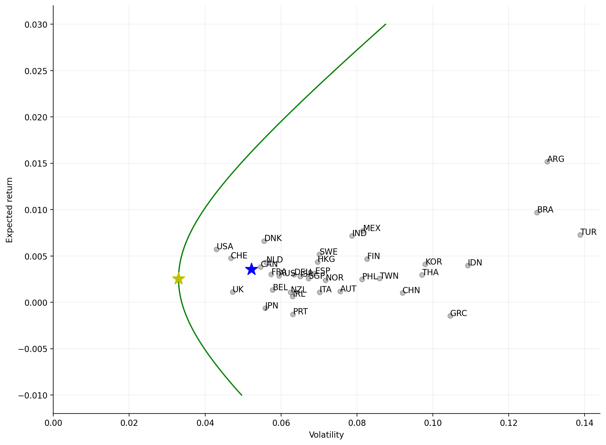
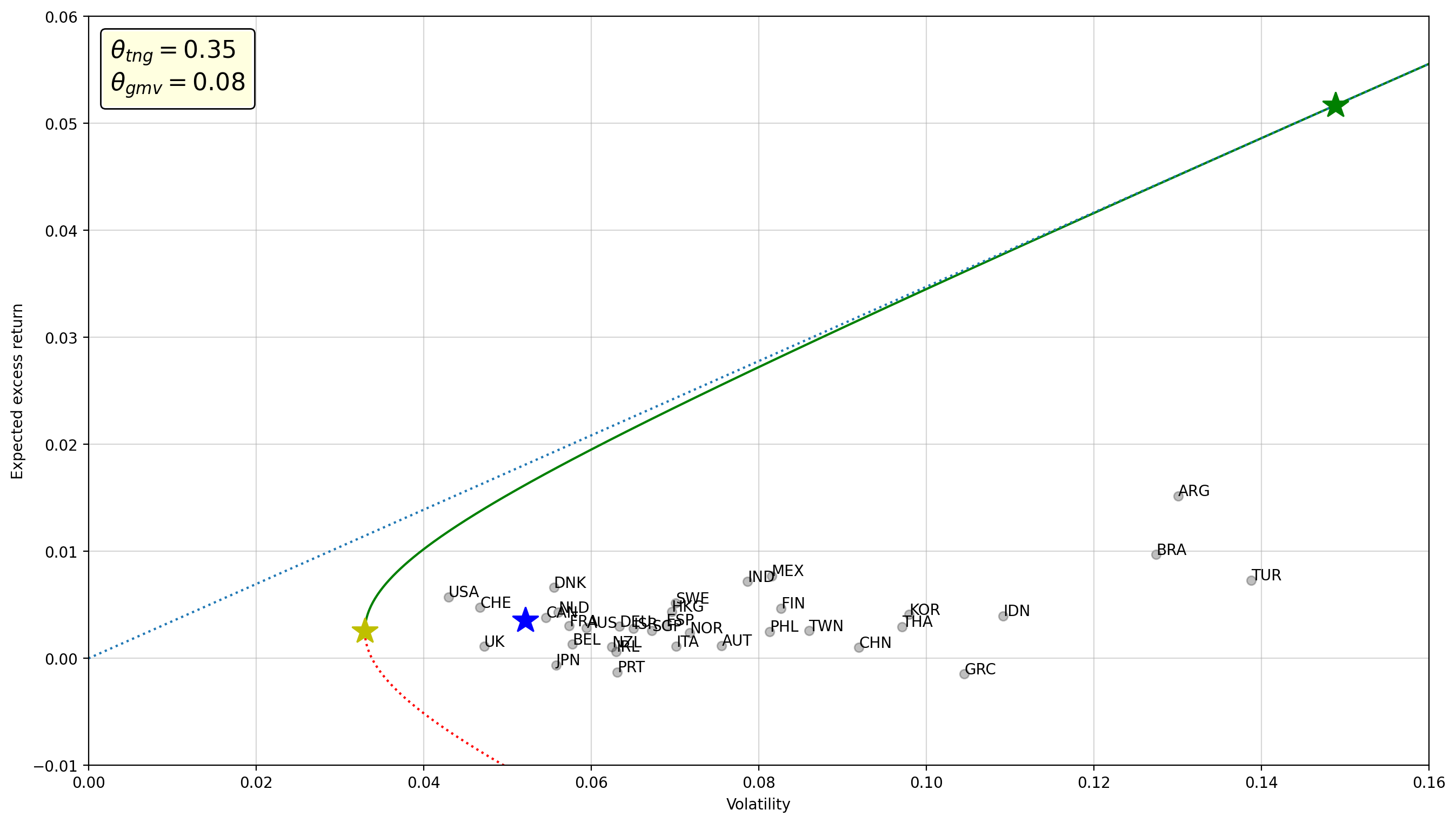
plot_frontier(rets)

Check your understanding

Is the Sharpe ratio of a portfolio shown on this graph? Where can we see the Sharpe ratio for the tangency portfolio?

Since we created a function to make this chart, it’s easy to see how altering the set of countries in the investment opportunity set changes the result.

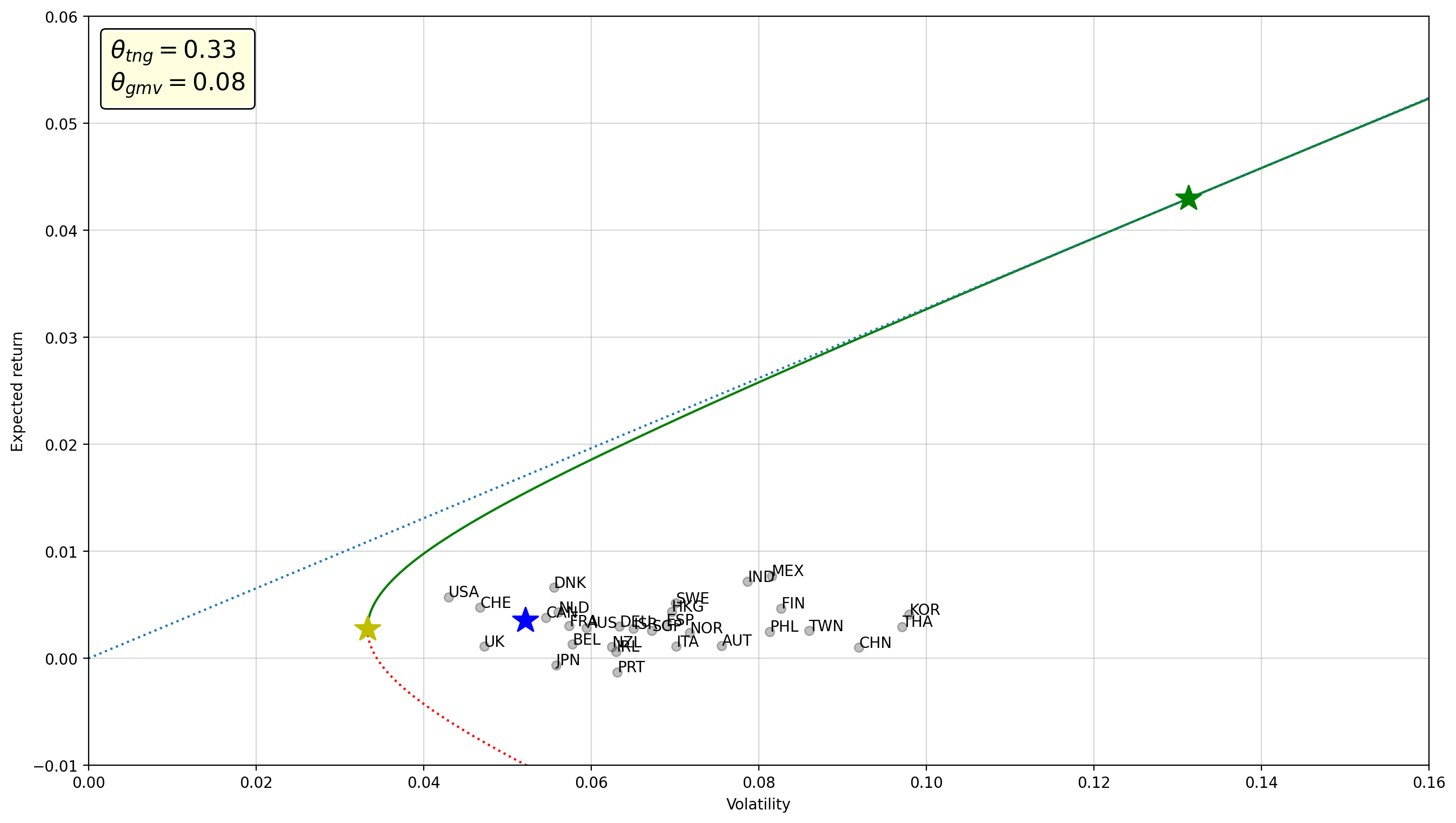
plot_frontier(rets.drop(columns=['Turkey', 'Brazil', 'Argentina', 'Greece', 'Indonesia']))

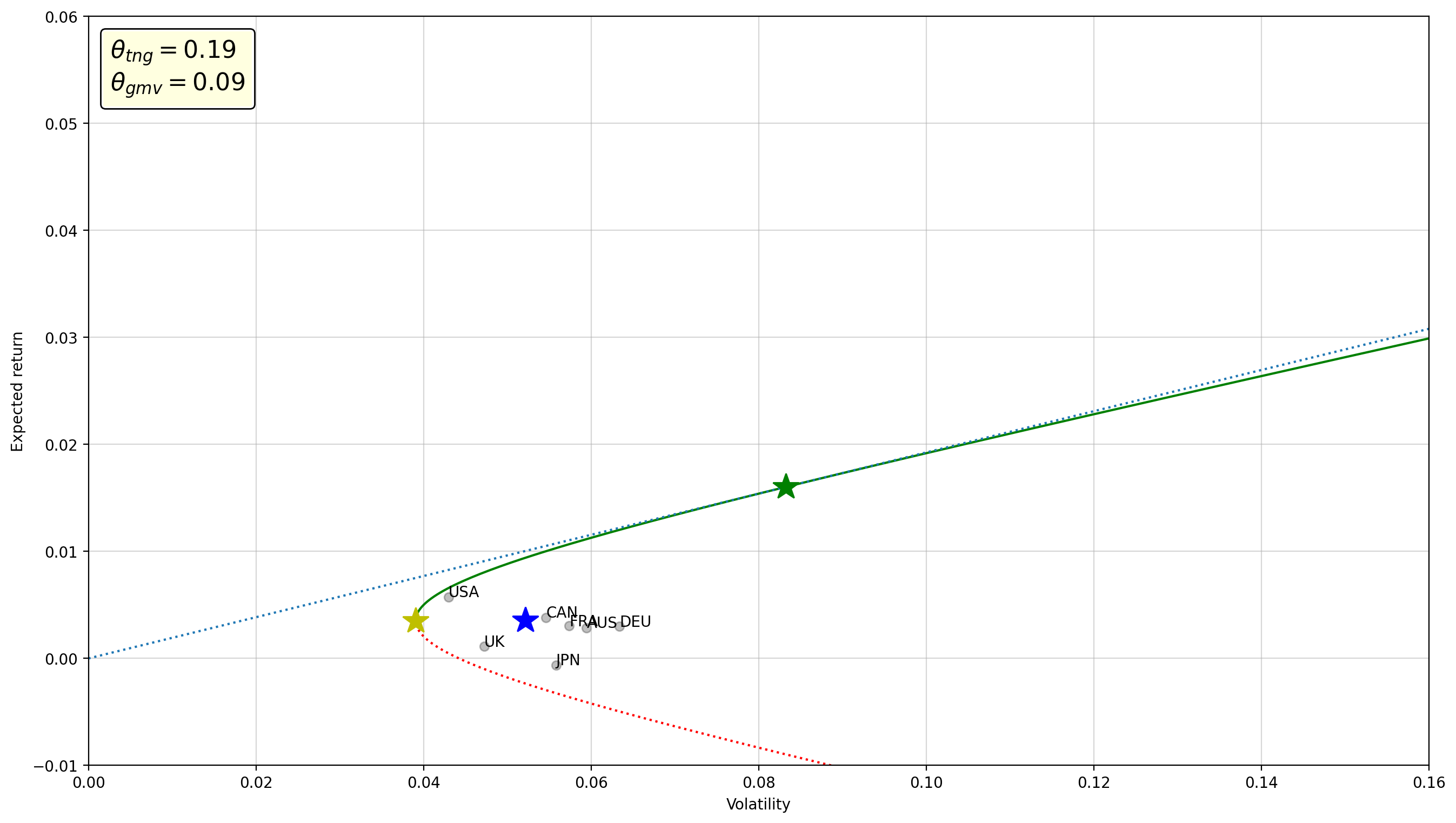
plot_frontier(rets[['USA', 'United Kingdom', 'Canada', 'Germany', 'France', 'Australia', 'Japan']])

Relationships between the TNG, GMV, and EW portfolios

As we saw above, the weights of the tangency portfolio are

\[\boldsymbol{\omega}_{\text{tng}} = \frac{\boldsymbol{\Sigma}^{-1} \boldsymbol{\mu}}{B} = \frac{\boldsymbol{\Sigma}^{-1} \boldsymbol{\mu}}{\mathbf{1}'\boldsymbol{\Sigma}^{-1} \boldsymbol{\mu}}.\]

If we assume that all assets have the same expected return, \(\mu\), then the vector of returns is

\[\begin{split}\boldsymbol{\mu} = \mu \cdot \begin{pmatrix}1 \\ \vdots \\ 1\end{pmatrix} = \mu \mathbf{1}.\end{split}\]

The weights therefore become

\[\boldsymbol{\omega}_{\text{tng}} = \frac{\boldsymbol{\Sigma}^{-1} \mu\mathbf{1}}{\mathbf{1}'\boldsymbol{\Sigma}^{-1} \mu\mathbf{1}} = \frac{\boldsymbol{\Sigma}^{-1} \mathbf{1}}{\mathbf{1}'\boldsymbol{\Sigma}^{-1} \mathbf{1}} = \boldsymbol{\omega}_{\text{gmv}}.\]

That is, the GMV portfolio is equivalent to the tangency portfolio if we assume that all expected returns are the same.

Next, consider the extreme case where all assets are uncorrelated and have the same variance. The covariance matrix is therefore simply

\[\begin{split}\boldsymbol{\Sigma} = \begin{pmatrix} \sigma^2 & 0 & \cdots & 0 \\ 0 & \sigma^2 & 0 & \vdots \\ 0 & 0 &\ddots & 0 \\ 0 & 0 & \cdots & \sigma^2 \\ \end{pmatrix} = \sigma^2 \bf{I},\end{split}\]

where the common variance is given by the constant \(\sigma^2\). In this case, the weights in the GMV are

\[\boldsymbol{\omega}_{\text{gmv}} = \frac{\boldsymbol{\Sigma}^{-1} \mathbf{1}}{\mathbf{1}'\boldsymbol{\Sigma}^{-1} \mathbf{1}} = \frac{(\sigma^2\bf{I})^{-1} \mathbf{1}}{\mathbf{1}'(\sigma^2\bf{I})^{-1} \mathbf{1}} = \frac{\mathbf{1}}{\mathbf{1}'\mathbf{1}} = \left(\frac{1}{N}, \frac{1}{N}, \ldots, \frac{1}{N}\right)' = \boldsymbol{\omega}_{\text{ew}}\]

That is, the GMV is equivlent to the equal-weighted portfolio in this case.

We can therefore think of the the equal-weighted portfolio as a special case of the global minimum variance portfolio, and the global minimum variance portfolio as a special case of the tangency portfolio. That is,

• the EW portfolio requires no estimates of expected returns, covariances, or variances;

• the GMV does use information about variances and covariances, but requires no estimates of expected returns; and

• the tangency portfolio requires estimates of all three.

The fact that the GMV can be calculated using estimates of only variances/covariances is important because it is actually a lot harder to estimate expected returns than it is to estimate the covariance matrix, as shown by Merton [1980]. We can collect more high-frequency data about returns to get more accurate estimates of variances and covariances, but sampling data with higher frequency does nothing to tell us more about the expected return. All we can do is wait for more time to pass to get more data and improve our estimate of the expected return.

If instead we assume that all assets have the same variance and a single correlation, we can write the variance–covariance matrix like this:

\[\begin{split}\boldsymbol{\Sigma} = \sigma^2 \begin{pmatrix} 1 & \rho & \cdots & \rho \\ \rho & 1 & \ddots & \rho \\ \vdots & \cdots & \ddots & \vdots \\ \rho & \cdots & \rho & 1 \\ \end{pmatrix}.\end{split}\]

In this case it can be shown that the GMV weights are

\[\omega_{\text{gmv}} = \frac{\boldsymbol{\Sigma}^{-1}\mathbf{1}}{\mathbf{1}'\boldsymbol{\Sigma}^{-1}\mathbf{1}} = \left(\frac{1}{N}, \cdots, \frac{1}{N}\right)' = \omega_{\text{ew}}.\]

Extra credit

To see this relationship, we start with the inverse of this variance–covariance matrix, which can be shown to be

\[\begin{split}\boldsymbol{\Sigma}^{-1} = \frac{1}{\sigma^2}\cdot\frac{1}{[(N-1)\rho+1](\rho-1)}\begin{pmatrix}-(N-2)\rho-1 & \rho & \cdots & \rho \\\rho & -(N-2)\rho-1 & \ddots & \rho \\\vdots & \cdots & \ddots & \vdots \\\rho & \cdots & \rho & -(N-2)\rho-1 \\\end{pmatrix}.\end{split}\]

The matrix part simply has \(\rho\) in all the off-diagonal terms, and \(-(N-2)\rho-1\) along the diagonal.

For example, in the \(N=2\) case, this is

\[\begin{split}\boldsymbol{\Sigma}^{-1} = \frac{1}{\sigma^2}\cdot\frac{1}{(\rho+1)(\rho-1)} \begin{pmatrix} -1 & \rho \\ \rho & -1 \\ \end{pmatrix}.\end{split}\]

Now, to calculate \(\boldsymbol{\Sigma}^{-1}\mathbf{1}\), we know that the result will be an \(N\times 1\) vector where each value is the sum of each row in \(\boldsymbol{\Sigma}^{-1}\). Each of these sums is the same: we have \(N-1\) terms with \(\rho\), plus the \(-(N-2)\rho-1\) term, so every row is

\[\frac{1}{\sigma^2} \frac{(N-1)\rho - (N-2)\rho-1}{[(N-1)\rho+1](\rho-1)} = \frac{1}{\sigma^2}\frac{1}{(N-1)\rho+1}.\]

That is,

\[\boldsymbol{\Sigma}^{-1}\mathbf{1} = \frac{1}{\sigma^2} \left(\frac{1}{(N-1)\rho + 1}, \quad \cdots, \quad \frac{1}{(N-1)\rho + 1} \right)'.\]

Now, \(\mathbf{1}'\boldsymbol{\Sigma}^{-1}\mathbf{1}\) is just the sum of these \(N\) values:

\[\mathbf{1}'\boldsymbol{\Sigma}^{-1}\mathbf{1} = \frac{1}{\sigma^2} \frac{N}{(N-1)\rho + 1}.\]

Therefore, the GMV weights are

\[\omega_{\text{gmv}} = \frac{\boldsymbol{\Sigma}^{-1}\mathbf{1}}{\mathbf{1}'\boldsymbol{\Sigma}^{-1}\mathbf{1}} = \left(\frac{1}{N}, \cdots, \frac{1}{N}\right)' = \omega_{\text{ew}}.\]

Of course, we need no information about either of the parameters, \(\sigma\) and \(\rho\), to calculate the equal-weight portfolio. So if we assume that these are the only two parameters in the covariance matrix, it no longer matters what they are. Whatever they are, they have no effect on the weights of the GMV, and estimating them becomes irrelevant. We simply end up with the equal-weighted portfolio.

Choosing particular values for \(N\), \(\sigma\), and \(\rho\), we see that the GMV weights are indeed those of an equal-weighted portfolio. Experiment by changing the inputs to see for yourself.

Portfolio weights

The index weights for the tangency and GMV portfolios are given here:

w_tng = Σinv @ μ / B
w_gmv = Σinv @ np.ones(N) / C

pd.DataFrame({'tng': w_tng,
              'gmv': w_gmv},
             index=rets.columns).sort_values('tng', ascending=False)

	tng	gmv
USA	2.861860	0.609641
Denmark	1.887925	0.131705
Switzerland	1.748860	0.258246
Hong Kong	0.902527	0.020683
Spain	0.863541	-0.088113
France	0.705587	-0.024290
India	0.621656	0.059804
Netherlands	0.479715	-0.233571
Argentina	0.318018	-0.005174
Austria	0.224530	-0.080220
Turkey	0.182038	-0.005140
Australia	0.176126	-0.034069
Korea	0.156850	-0.068463
Brazil	0.150849	-0.038806
Finland	0.071142	-0.035367
Mexico	0.032842	-0.008054
Sweden	-0.011616	-0.164743
Thailand	-0.036107	-0.024262
Singapore	-0.084327	-0.079599
Indonesia	-0.086577	-0.006827
Taiwan	-0.170203	0.060319
Canada	-0.197325	-0.034822
Philippines	-0.234042	0.042504
Greece	-0.320697	-0.018502
Norway	-0.336597	-0.108096
Ireland	-0.364012	-0.075121
New Zealand	-0.453692	0.081240
Italy	-0.517786	0.095383
China	-0.565748	0.040135
Israel	-0.708202	0.091107
Belgium	-0.796391	0.059256
Germany	-0.923938	-0.150510
Japan	-1.048085	0.185264
Portugal	-1.390965	0.140258
United Kingdom	-2.137757	0.408204