Time series models

import numpy as np
import pandas as pd
import matplotlib.pyplot as plt
import wrds

db = wrds.Connection()

Loading library list...
Done

White noise

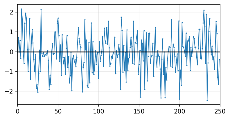
A time series is said to be white noise if its realizations are drawn from an iid (independent and identically distributed) random variable. A special case is Gaussian white noise, where

\[\varepsilon_t \overset{iid}{\sim} \N(0, \sigma_{\varepsilon}^2).\]

This assumption has three implications:

1. \(\E(\varepsilon_t) = \E(\varepsilon_t | \varepsilon_{t-1}, \varepsilon_{t-2}, \ldots) = 0\),

2. \(\E(\varepsilon_t \varepsilon_{t-j}) = \cov(\varepsilon_{t}, \varepsilon_{t-j}) = 0\),

3. \(\var(\varepsilon_t) = \var(\varepsilon_t | \varepsilon_{t-1}, \varepsilon_{t-2}, \ldots) = \sigma_{\varepsilon}^2\).

The first and second facts imply the absense of any serial correlation or predictability. The third fact implies that the series is conditionally homoskedastic, or has a constant conditional variance, where “conditional” means that we use what we know about how the time series has behaved up until a point in time.

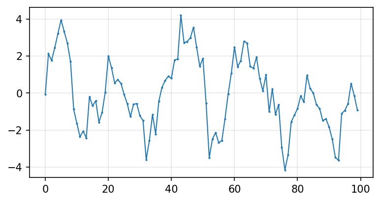
rng = np.random.default_rng(8675309)

T = 250
ε = rng.standard_normal(T)

fig, ax = plt.subplots(figsize=(6,3))
ax.plot(ε, lw=1, marker='.', markersize=2)

ax.set_xlim(0,T)
ax.grid(alpha=0.3)
ax.hlines(0, xmin=0, xmax=T, color='k')
plt.show()

We can construct more complex models of time series by taking linear combinations of white noise:

Type	Equation
AR(1)	\(x_t = \phi x_{t-1} + \varepsilon_t\)
AR(p)	\(x_t = \phi_1 x_{t-1} + \phi_2 x_{t-2} + \cdots + \phi_p x_{t-p} +\varepsilon_t\)
MA(1)	\(x_t = \varepsilon_t + \theta \varepsilon_{t-1}\)
MA(q)	\(x_t = \varepsilon_t + \theta_1 \varepsilon_{t-1} + \theta_2 \varepsilon_{t-2} + \cdots + \theta_q \varepsilon_{t-q}\)
ARMA(p,q)	\(x_t = \phi_1 x_{t-1} + \cdots + \phi_p x_{t-p} + \varepsilon_t + \theta_1 \varepsilon_{t-1} + \cdots + \theta_q \varepsilon_{t-q}\)

Adding a constant to the model will absorb any mean in the underlying process. To see this, suppose that the demeaned value of \(x\) follows an AR(1), so

\[x_t - \bar x = \phi (x_{t-1} - \bar x) + \varepsilon_t.\]

This is the same thing as

\[x_t = (1 - \phi)\bar x + \phi x_{t-1} + \varepsilon_t\]

which is simply an AR(1) with an added constant term, \(\phi_0 := (1-\phi)\bar x\). In other words, if we specify a model with a constant term it is equivalent to first subtracting the mean from the series.

Stationarity

A times series is said to be weakly stationary if

• \(\E(r_t) = \mu\); and

• \(\cov(r_t,r_{t-k})=\gamma_k\).

That is, the expected return is constant over time, and the covariance between the return at time \(t\) and time \(t-k\) depends only on the horizon \(k\), not on where in the time series we are, \(t\).

Autocorrelation function (ACF)

We will define the autocovariance of a time series \(\{r_t\}\) with \(k\) lags as

\[\gamma_k := \cov(r_t, r_{t-k}).\]

That is, what is the covariance of a series with itself where we compare the value at time \(t\) with the value at some earlier time \(t-k\). Note that it follows immediately that \(\gamma_0 = \var(r_t).\)

Recall that the correlation coefficient between two random variables \(X\) and \(Y\) is defined as

\[\rho_{X,Y} = \frac{\cov(X,Y)}{\sqrt{\var(X)\var(Y)}} = \frac{\cov(X,Y)}{\sigma_X \sigma_Y}.\]

The correlation between \(r_t\) and \(r_{t-k}\) is therefore

\[\rho(k) = \frac{\cov(r_t,r_{t-k})}{\sqrt{\var(r_t)\var(r_{t-k})}} = \frac{\cov(r_t,r_{t-k})}{\var(r)} = \frac{\gamma_k}{\gamma_0}.\]

Notice that this definition assumes the series is weakly stationary, so \(\var(r_t) = \var(r_{t-k}) = \var(r)\).

\(\rho(k)\) is the autocorrelation function. It gives the autocorrelation for a time series as a function of \(k\).

Let’s calculate \(\rho(1)\) for S&P 500 index using the last ten years of daily data. We’ll multiply by 100 to avoid precision problems later.

sp500 = db.get_table('crsp', 'dsp500', date_cols=['caldt'], columns=['caldt', 'spindx']).set_index('caldt')

sp500 = sp500.dropna().squeeze()

rets = sp500.loc['2014':].pct_change().dropna() * 100

rets

caldt
2014-01-03   -0.033297
2014-01-06   -0.251178
2014-01-07    0.608177
2014-01-08    -0.02122
2014-01-09     0.03483
                ...   
2024-12-24    1.104272
2024-12-26   -0.040563
2024-12-27   -1.105574
2024-12-30   -1.070201
2024-12-31   -0.428479
Name: spindx, Length: 2767, dtype: Float64

# calculate the 1-period autocovariance
covmat = np.cov(rets[:-1], rets[1:])
covmat

array([[ 1.19287291, -0.15691324],
       [-0.15691324,  1.1929527 ]])

# 1-period autocorrelation
covmat[0,1] / covmat[0,0]

-0.13154229872535833

The ACF is built-in to the statsmodels library, along with a helpful plotting function.

import statsmodels.api as sm
from statsmodels.tsa import stattools as st

st.acf(rets, nlags=10)

array([ 1.        , -0.13153323,  0.07357237, -0.01855214, -0.06314426,
        0.04068317, -0.11227941,  0.1431176 , -0.12037467,  0.12920954,
       -0.06164976])

fig, ax = plt.subplots(figsize=(6,3))

fig = sm.graphics.tsa.plot_acf(rets, lags=25, ax=ax)

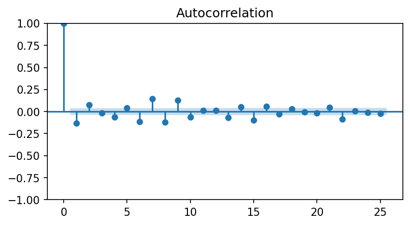
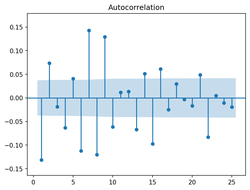
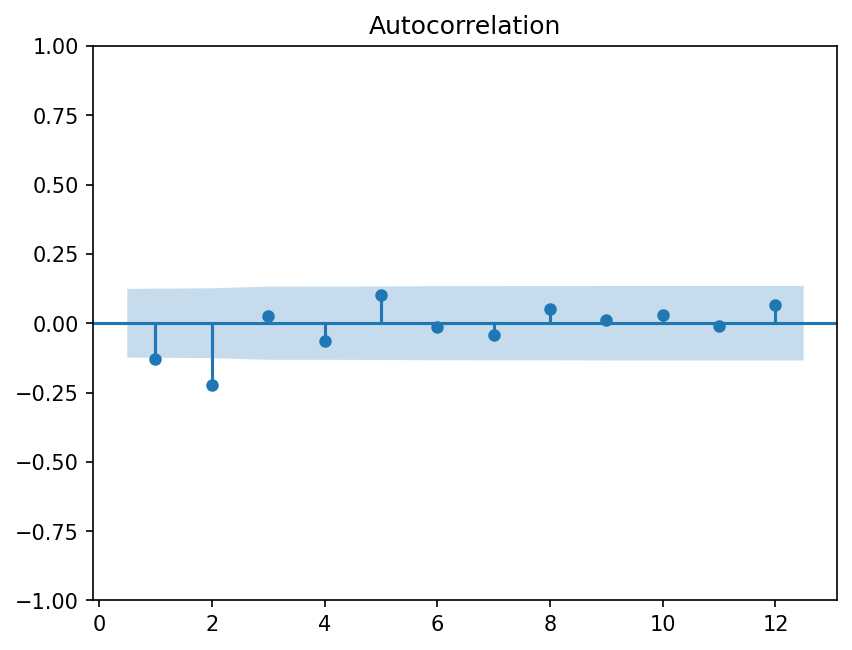
Since \(\rho(1)\) is always equal to one, it is common to plot the autocorrelation without this value.

fig = sm.graphics.tsa.plot_acf(rets, lags=25, zero=False, auto_ylims=True)

Testing for autocorrelation at multiple horizons is done using a portmanteau test such as the Ljung-Box statistic,

\[Q(m) = T(T+2)\sum_{k=1}^m \frac{\hat\rho(k)^2}{T-k}\]

where we choose some number \(m\) as the maximum number of lags to consider.

m = 5

acfs = st.acf(rets, nlags=m)

T = len(rets)
k = np.arange(1,len(acfs))

# Q(m) statistic
q = T * (T+2) * (acfs[1:]**2 / (T-k)).sum()
q

79.52483849195411

How do we interpret this value? Is it big? Small?

We need to know what we would expect it to be if there aren’t significant correlations. In other words, under the null hypothesis of no autocorrelation at all \(m\) lags, what is the distribution of the \(Q(m)\) statistic? How surprised should we be at seeing a number like 149?

Ljung and Box (1978) showed that under the null of no autocorrelations, the test statistic has a \(\chi^2\) distribution with \(m\) degrees of freedom.

If \(Q\) is larger than \(\chi^2_{\alpha}\) then we reject the null at the \(\alpha\) significance level. For example, the cutoff for a 5% test is about 11.

from scipy.stats import chi2

chi2.ppf(0.95, df=m)

11.070497693516351

Clearly, the \(Q\) statistic we calculated is far greater than this value, indicating that we can easily reject the null hypothesis.

By specifying qstat=True we get \(Q\)-statistics with corresponding \(p\)-values. (Recall that a \(p\)-value is the probability of observing a statistic of some magnitude under the null hypothesis. In this case, the null hypothesis is that there is no serial correlation. If the test-statistic is larger than the corresponding “critical value” then the probability of getting this result if the null hypothesis is true is small. We take this as evidence against the null.)

acf, qstats, pvals = st.acf(rets, nlags=10, qstat=True)

qstats

array([ 47.92376387,  62.92290611,  63.87698069,  74.93351291,
        79.52483849, 114.50855801, 171.36885614, 211.60817794,
       257.98778164, 268.55007335])

pvals

array([4.43118117e-12, 2.17002404e-14, 8.72063582e-14, 2.05816403e-15,
       1.05499815e-15, 2.31492106e-22, 1.29154929e-33, 2.27821811e-41,
       2.05052164e-50, 6.75920631e-52])

AR models

from statsmodels.tsa.arima_process import ArmaProcess, arma_acf
from statsmodels.tsa.arima.model import ARIMA

Suppose returns, \(r_t\), follow and AR(1) model,

\[r_t = \phi_0 + \phi_1 r_{t-1} + \varepsilon_t.\]

We can calculate conditional mean and variance of \(r_t\) as

\[\E(r_t|r_{t-1}) = \phi_0 + \phi_1 r_{t-1}\]

and

\[\var(r_t|r_{t-1}) = \var(\varepsilon_t) = \sigma^2_{\varepsilon}.\]

To find the unconditional mean, begin by taking the expectation of each side of the equation:

\[\begin{split} \begin{aligned} \E(r_t) &= \phi_0 + \phi_1 \E(r_{t-1}) \\ \Longrightarrow\E(r_t) &= \frac{\phi_0}{1 - \phi_1}. \end{aligned} \end{split}\]

Notice that this result requires the stationarity assumption so \(\E(r_t) = \E(r_{t-1}).\) Similarly, the variance is

\[\begin{split} \begin{aligned} \var(r_t) &= \phi_1^2\var(r_{t-1}) + \sigma^2_{\varepsilon} \\ \Longrightarrow \var(r_t) &= \frac{\sigma^2_{\varepsilon}}{1 - \phi_1^2}. \end{aligned} \end{split}\]

In the more general case of the AR(p) model, the unconditional mean is

\[\E(r_t) = \frac{\phi_0}{1-\sum_{i=1}^p \phi_i}.\]

The unconditional variance is more complicated to solve in the general case because there are covariance terms that complicate the math and require a recursive solution procedure.

We can simulate an AR(p) process as follows:

def simulate_ar1(φ0, φ1, T=1000):
    rng = np.random.default_rng()
    
    # initilize series
    r = np.zeros(T+1)

    # simulate AR(1) process with forward recursion
    ε = rng.standard_normal(T+1)
    for t in range(1,T+1):
        r[t]  = φ0 + φ1*r[t-1] + ε[t]

    # return the series without the initial value
    return r[1:]

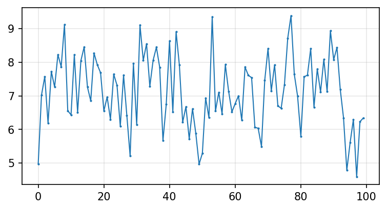
r = simulate_ar1(5, .3)

print('Theoretical mean: {:0.3f}'.format(5/(1-.3)))
print('Sample mean: {:0.3f}'.format(r.mean()))

print('Theoretical variance: {:0.3f}'.format(1/(1-.3**2)))
print('Sample variance: {:0.3f}'.format(r.var()))

Theoretical mean: 7.143
Sample mean: 7.078
Theoretical variance: 1.099
Sample variance: 1.077

# plot the first 100 observations
fig, ax = plt.subplots(figsize=(6,3))
ax.plot(r[:100], lw=1, marker='.', markersize=2)
ax.grid(alpha=0.3)

r = simulate_ar1(0, .8)

fig, ax = plt.subplots(figsize=(6,3))
ax.plot(r[:100], lw=1, marker='.', markersize=2)
ax.grid(alpha=0.3)

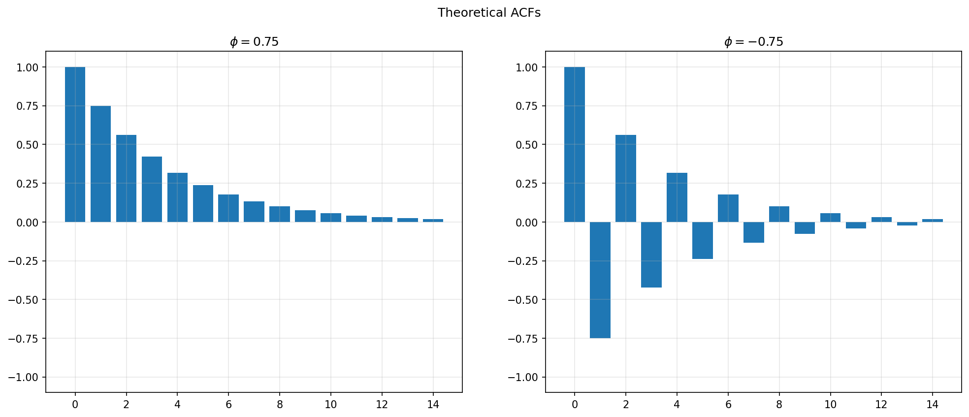
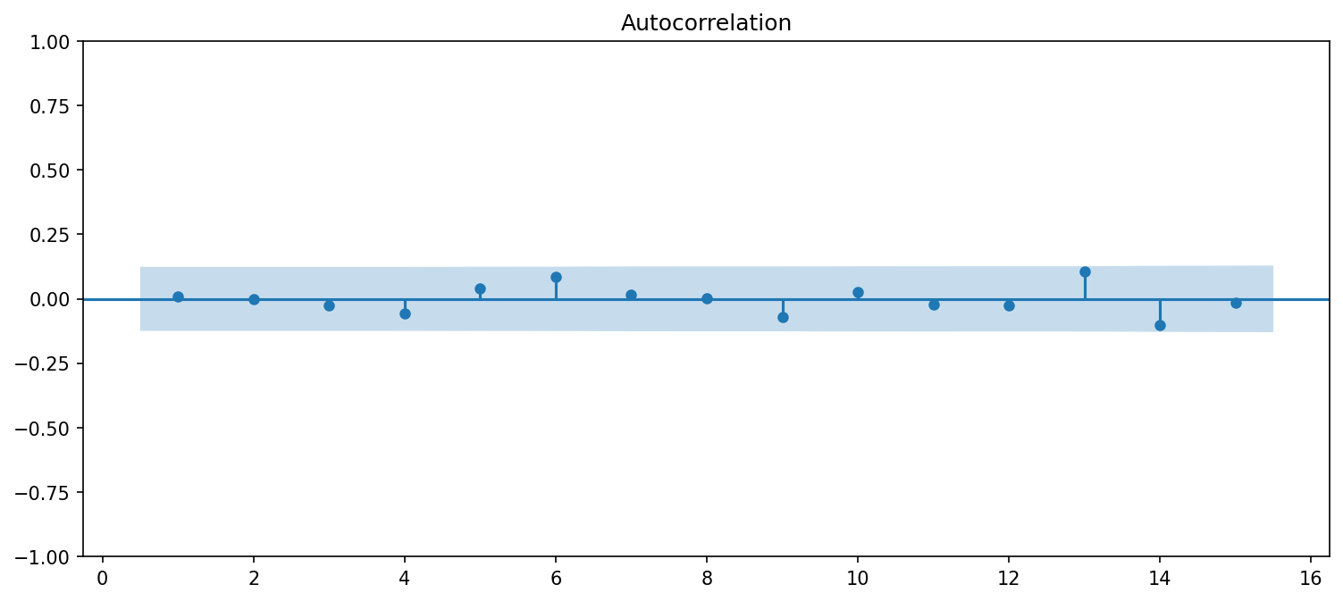
Consider the plot of the ACF for two different AR(1) models: one with \(\phi=0.75\) and the other with \(\phi=-0.75\).

Show code cell source

Hide code cell source

φ = 0.75
lags = 15

fig, (ax1, ax2) = plt.subplots(1,2,figsize=(16,6))

# AR(1) process with φ = 0.75
acf = arma_acf([1, -φ], [1], lags=lags)
ax1.bar(np.arange(lags), acf)
ax1.set_title(rf'$\phi={φ}$')

# AR(1) process with φ = -0.75
acf = arma_acf([1, φ], [1], lags=lags)
ax2.bar(np.arange(lags), acf)
ax2.set_title(rf'$\phi={-φ}$')

for ax in (ax1, ax2):
    ax.set_ylim((-1.1,1.1))
    ax.grid(alpha=0.3)

fig.suptitle('Theoretical ACFs')
plt.show()

Clearly the autocorrelations for an AR process die out as \(k\) increases. To see why, notice that the model

\[r_t = \phi r_{t-1} + \varepsilon_t\]

means that of course

\[r_{t-1} = \phi r_{t-2} + \varepsilon_{t-1}.\]

We can then calculate \(\gamma_1\):

\[\begin{split} \begin{align*} \cov(r_t,r_{t-1}) &= \cov(\phi r_{t-1} + \varepsilon_t, r_{t-1}) \\ &= \cov(\phi r_{t-1}, r_{t-1}) + \cov(\varepsilon_t, r_{t-1}) \\ &= \phi\cov(r_{t-1}, r_{t-1}) + \cov(\varepsilon_t, r_{t-1}) \\ &= \phi\var(r), \end{align*} \end{split}\]

and therefore \(\rho(1) = \phi\).

But notice also that, by subsituting the value for \(r_{t-1}\) into the first equation,

\[\begin{split} \begin{align*} r_t &= \phi (\phi r_{t-2} + \varepsilon_{t-1}) + \varepsilon_t, \\ &= \phi^2 r_{t-2} + \phi\varepsilon_{t-1} + \varepsilon_t. \end{align*} \end{split}\]

This implies that \(\rho(2) = \phi^2\).

But we don’t have to stop there. We could do the same recursion again, which gives

\[ \begin{equation*} r_t = \phi^3 r_{t-3} + \phi^2\varepsilon_{t-2} + \phi\varepsilon_{t-1} + \varepsilon_t, \end{equation*} \]

implying that \(\rho(3) = \phi^3\).

Repeating this recursion ad infinitum leads to the general result that

\[r_t = \phi^k r_{t-k} + \sum_{i=0}^{k-1}\phi^i \varepsilon_{t-i},\]

so

\[\rho(k) = \phi^k.\]

So, as we see in the graph above, when \(\phi=0.75\) we’ll find:

• \(\rho(1) = 0.75\)

• \(\rho(2) = 0.75^2 \approx 0.56\)

• \(\rho(3) = 0.75^3 \approx 0.42\)

and so on.

As we take \(k\rightarrow\infty\), the first term disappears because \(\phi<1\). We’ll see below that this means we are left with an MA model where \(q=\infty\). In other words, an AR(1) model is equivalent to an MA(\(\infty\)) model.

While we can simulate series as we did above, the ArmaProcess function provides a built-in functionality to do this kind of simulation, and also works with other types of time series models.

φ = 0.75
T = 250

y = ArmaProcess([1, -φ]).generate_sample(T)

Show code cell source

Hide code cell source

fig, ax = plt.subplots()
ax.plot(y, lw=1, marker='.', markersize=2)
ax.grid(alpha=0.3)
ax.set_xlim(0,T)
ax.set_title('Simulated data')
plt.show()

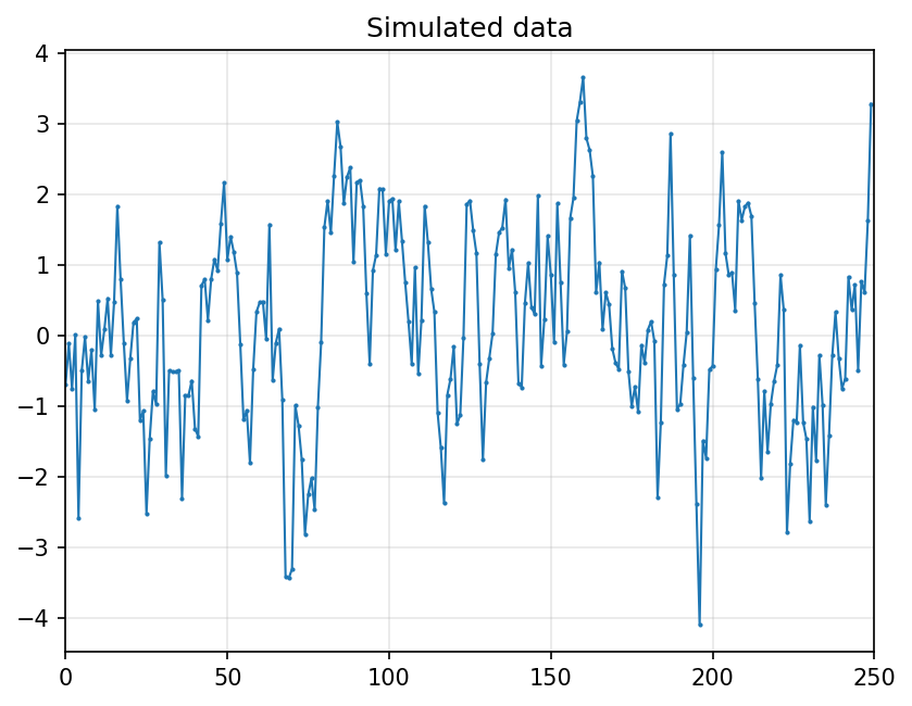
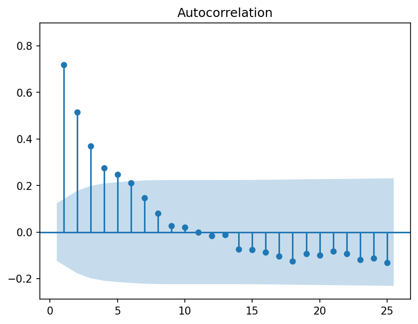
fig = sm.graphics.tsa.plot_acf(y, lags=25, zero=False, auto_ylims=True)

Estimating AR coefficients

We can estimate the \(\phi\) parameters using OLS.

res_ols = sm.OLS(y[1:], sm.add_constant(y[:-1])).fit()

print(res_ols.summary())

                            OLS Regression Results                            
==============================================================================
Dep. Variable:                      y   R-squared:                       0.528
Model:                            OLS   Adj. R-squared:                  0.526
Method:                 Least Squares   F-statistic:                     276.3
Date:                Mon, 06 Apr 2026   Prob (F-statistic):           3.78e-42
Time:                        14:49:40   Log-Likelihood:                -344.37
No. Observations:                 249   AIC:                             692.7
Df Residuals:                     247   BIC:                             699.8
Df Model:                           1                                         
Covariance Type:            nonrobust                                         
==============================================================================
                 coef    std err          t      P>|t|      [0.025      0.975]
------------------------------------------------------------------------------
const          0.0432      0.062      0.702      0.483      -0.078       0.164
x1             0.7337      0.044     16.621      0.000       0.647       0.821
==============================================================================
Omnibus:                        6.007   Durbin-Watson:                   1.966
Prob(Omnibus):                  0.050   Jarque-Bera (JB):                5.846
Skew:                          -0.372   Prob(JB):                       0.0538
Kurtosis:                       3.098   Cond. No.                         1.41
==============================================================================

Notes:
[1] Standard Errors assume that the covariance matrix of the errors is correctly specified.

A better way to fit a model like this uses AugtoReg.

from statsmodels.tsa.ar_model import AutoReg, ar_select_order

res = AutoReg(y, lags=1, trend='c').fit()
print(res.summary())

                            AutoReg Model Results                             
==============================================================================
Dep. Variable:                      y   No. Observations:                  250
Model:                     AutoReg(1)   Log Likelihood                -344.371
Method:               Conditional MLE   S.D. of innovations              0.965
Date:                Mon, 06 Apr 2026   AIC                            694.742
Time:                        14:49:42   BIC                            705.294
Sample:                             1   HQIC                           698.989
                                  250                                         
==============================================================================
                 coef    std err          z      P>|z|      [0.025      0.975]
------------------------------------------------------------------------------
const          0.0432      0.061      0.705      0.481      -0.077       0.163
y.L1           0.7337      0.044     16.689      0.000       0.648       0.820
                                    Roots                                    
=============================================================================
                  Real          Imaginary           Modulus         Frequency
-----------------------------------------------------------------------------
AR.1            1.3630           +0.0000j            1.3630            0.0000
-----------------------------------------------------------------------------

Show code cell source

Hide code cell source

fig, ax = plt.subplots(figsize=(10,4))
ax.plot(res.resid, lw=1, marker='.', markersize=2)
ax.set_title('Residuals')
ax.grid(alpha=0.3)
plt.show()

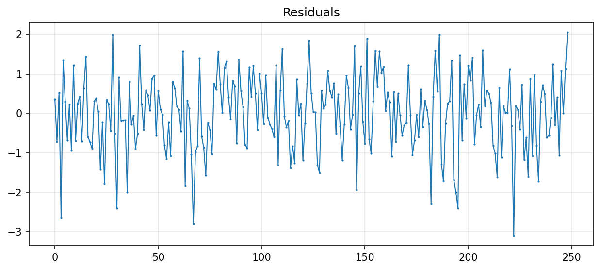
fig, ax = plt.subplots(figsize=(12,5))
fig = sm.graphics.tsa.plot_acf(res.resid, lags=15, zero=False, ax=ax)

Partial autocorrelation function (PACF)

With real data we don’t know the correct \(p\) and must estimate it. This can be done using the Partial Autocorrelation Function (PACF).

Consider this sequence of regressions, where we add one more lag to each subsequent regression:

\[\begin{split}\begin{align*} r_t &= \phi_{0,1} + \textcolor{blue}{\phi_{1,1}} r_{t-1} + \varepsilon_{1t} \\ r_t &= \phi_{0,2} + \phi_{1,2} r_{t-1} + \textcolor{blue}{\phi_{2,2}} r_{t-2} + \varepsilon_{2t} \\ r_t &= \phi_{0,3} + \phi_{1,3} r_{t-1} + \phi_{2,3} r_{t-2} + \textcolor{blue}{\phi_{3,3}} r_{t-3} + \varepsilon_{3t} \\ r_t &= \phi_{0,4} + \phi_{1,4} r_{t-1} + \phi_{2,4} r_{t-2} + \phi_{3,4} r_{t-3} + \textcolor{blue}{\phi_{4,4}} r_{t-4} + \varepsilon_{3t} \\ &\vdots \end{align*}\end{split}\]

The terms \(\phi_{1,1}, \phi_{2,2}, \phi_{3,3}, \phi_{4,4}, \ldots\) are the relevant coefficients. Each gives the marginal effect of adding one additional lag to the autoregression.

Estimating these regressions using OLS, we get estimates for the \(\phi\), which have these properties:

• \(\hat \phi_{p,p}\) converges to \(\phi_p\) as \(T\rightarrow \infty\); and

• \(\hat \phi_{k,k}\) converges to zero for all \(k>p\).

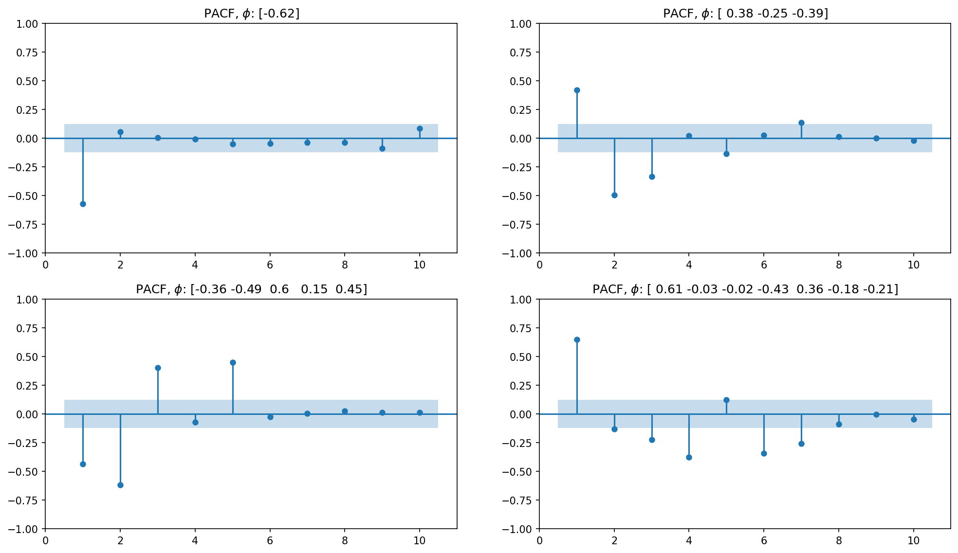
This means that we can determine \(p\) by looking at where the PACF drops off. For example, consider these figures:

Show code cell source

Hide code cell source

def get_rand_coefs(p):
    '''Generate coefficients for a stationary AR(p) model'''
    from statsmodels.tsa.statespace.tools import is_invertible
    rng = np.random.default_rng()
    while True:
        coefs = rng.uniform(-.95,.95,p).round(2)
        if np.all(coefs != 0) and is_invertible(np.r_[1, -coefs]):
            return coefs

def simulate_ar(nlags=None, nobs=250, coefs=None):
    if coefs is None:
        coefs = get_rand_coefs(nlags)
    else:
        coefs = np.array(coefs)
    # simulate series
    return ArmaProcess(np.r_[1, -coefs]).generate_sample(nobs), coefs

φ = 0.5

# Plot PACF
fig, (ax1, ax2) = plt.subplots(1,2)

y,_ = simulate_ar(coefs=[φ])
fig = sm.graphics.tsa.plot_pacf(y, lags=10, ax=ax1, zero=None)
ax1.set_title(r'PACF, $\phi_1={}$'.format(φ))

y,_ = simulate_ar(coefs=[-𝜙])
fig = sm.graphics.tsa.plot_pacf(y, lags=10, ax=ax2, zero=None)
ax2.set_title(r'PACF, $\phi_1={}$'.format(-φ))

for ax in [ax1, ax2]:
    ax.set_ylim(-1.1, 1.1)

plt.show()

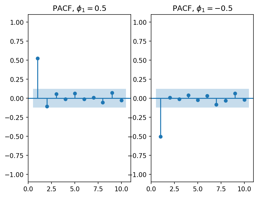
fig, axes = plt.subplots(2,2,figsize=(16,9))

lags = [1, 3, 5, 7]

for n,ax in zip(lags, axes.ravel()):
    y, params = simulate_ar(n)
    fig = sm.graphics.tsa.plot_pacf(y, lags=10, ax=ax, zero=None)
    ax.set_title(r'PACF, $\phi$: {}'.format(params))

Information criteria

We can select among different possible models by evaluating an information criterion. In particular, we can use either the Akaike information criterion (AIC) or the Schwarz-Bayesian information criterion (BIC). Both criteria begin with the log-likelihood function, which measures how likely we are to see the observed data given the model parameters we have estimated.

In the case of the autoregression model, the log-likelihood is given by

\[\ln \mathcal{L} = -\frac{T-\ell}{2} \left(\ln(2\pi) + \ln(\hat\sigma_{\varepsilon}^2)+1 \right),\]

where \(T\) is the number of time series observations, \(\ell\) is the number of lags in the model, and \(\hat\sigma_{\varepsilon}^2\) is the variance of the residuals. We can think of \(T-\ell\) as the effictive number of observations, since we lose one observation for each additional lag we include in the model.

Notice that this is smaller when the variance of the residuals, \(\hat\sigma_{\varepsilon}^2\), is greater. That is, the more variance our model leaves unexplained, the lower is the likelihood of the model, and the worse is its fit.

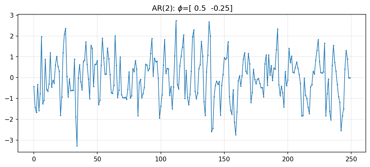
We’ll begin by simulating a new time series to work with.

y, params = simulate_ar(2, coefs=[0.5, -0.25])

fig, ax = plt.subplots(figsize=(10,4))
ax.plot(y, lw=1, marker='.', markersize=2)
ax.grid(alpha=0.3)
ax.set_title(r'AR({}): $\phi$={}'.format(len(params), params))
plt.show()

# fit AR(1) model

res = AutoReg(y, lags=1, trend='c').fit()
print(res.summary())

                            AutoReg Model Results                             
==============================================================================
Dep. Variable:                      y   No. Observations:                  250
Model:                     AutoReg(1)   Log Likelihood                -350.849
Method:               Conditional MLE   S.D. of innovations              0.990
Date:                Mon, 06 Apr 2026   AIC                            707.698
Time:                        14:57:22   BIC                            718.251
Sample:                             1   HQIC                           711.946
                                  250                                         
==============================================================================
                 coef    std err          z      P>|z|      [0.025      0.975]
------------------------------------------------------------------------------
const         -0.0145      0.063     -0.231      0.817      -0.138       0.109
y.L1           0.4229      0.057      7.367      0.000       0.310       0.535
                                    Roots                                    
=============================================================================
                  Real          Imaginary           Modulus         Frequency
-----------------------------------------------------------------------------
AR.1            2.3644           +0.0000j            2.3644            0.0000
-----------------------------------------------------------------------------

res.sigma2

0.9803828131430133

res.llf

-350.8490811049661

The AIC is then defined as

\[AIC = -2 \ln \mathcal{L} + 2(1+k),\]

where \(k\) is the degrees of freedom in the model, or the number of lags (plus one if there is a constant term).

We prefer models with a lower AIC. This happens when the likelihood is higher or when we have fewer parameters to estimate.

print('Volatility of residuals: {:.4f}'.format(np.sqrt(res.sigma2)))

print('Number of observations: {}'.format(res.nobs))

print('Degrees of freedom: {}'.format(res.df_model))

print('AIC: {:.3f}'.format(-2*res.llf + 2*(1+res.df_model)))

Volatility of residuals: 0.9901
Number of observations: 249
Degrees of freedom: 2
AIC: 707.698

res.aic

707.6981622099322

The BIC is defined as

\[BIC = -2 \ln \mathcal{L} + (1+k)\ln(T-\ell).\]

-2*res.llf + (res.df_model+1)*np.log(res.nobs)

718.2505208993264

res.bic

718.2505208993264

We can use AIC or BIC to aid in order selection.

modsel = ar_select_order(y, maxlag=6, old_names=False)

# best model appears first
modsel.aic

{(1, 2): 677.3421077542574,
 (1, 2, 3): 679.0364587384304,
 (1, 2, 3, 4): 680.3446488925334,
 (1, 2, 3, 4, 5): 682.3372111722496,
 (1, 2, 3, 4, 5, 6): 684.2853092734316,
 (1,): 691.5814367086749,
 0: 736.108125654351}

modsel.bic

{(1, 2): 687.833612430137,
 (1, 2, 3): 693.0251316396032,
 (1, 2, 3, 4): 697.8304900189994,
 (1,): 698.5757731592613,
 (1, 2, 3, 4, 5): 703.3202205240087,
 (1, 2, 3, 4, 5, 6): 708.765486850484,
 0: 739.6052938796443}

# number of lags selected by default selected criterion (default is BIC)
modsel.ar_lags

[1, 2]

areg = AutoReg(y, lags=2, trend='c', old_names=False).fit()
print(areg.summary())

                            AutoReg Model Results                             
==============================================================================
Dep. Variable:                      y   No. Observations:                  250
Model:                     AutoReg(2)   Log Likelihood                -341.577
Method:               Conditional MLE   S.D. of innovations              0.959
Date:                Mon, 06 Apr 2026   AIC                            691.153
Time:                        14:58:44   BIC                            705.207
Sample:                             2   HQIC                           696.811
                                  250                                         
==============================================================================
                 coef    std err          z      P>|z|      [0.025      0.975]
------------------------------------------------------------------------------
const         -0.0137      0.061     -0.224      0.823      -0.133       0.106
y.L1           0.5240      0.061      8.535      0.000       0.404       0.644
y.L2          -0.2426      0.061     -3.953      0.000      -0.363      -0.122
                                    Roots                                    
=============================================================================
                  Real          Imaginary           Modulus         Frequency
-----------------------------------------------------------------------------
AR.1            1.0797           -1.7191j            2.0301           -0.1607
AR.2            1.0797           +1.7191j            2.0301            0.1607
-----------------------------------------------------------------------------

Next, let’s look at the monthly return on the value-weighted market series. The series starts in 1926.

vwret = db.get_table('crsp', 'msi', columns=['date', 'vwretd'], date_cols=['date'])

vwret = vwret.dropna().set_index('date').squeeze()

# move dates to end of month to avoid warnings with model selection
vwret = vwret.asfreq('ME', method='ffill')

vwret

date
1926-01-31    0.000561
1926-02-28   -0.033046
1926-03-31   -0.064002
1926-04-30    0.037029
1926-05-31    0.012095
                ...   
2024-08-31    0.021572
2024-09-30    0.020969
2024-10-31   -0.008298
2024-11-30    0.064855
2024-12-31   -0.031582
Freq: ME, Name: vwretd, Length: 1188, dtype: Float64

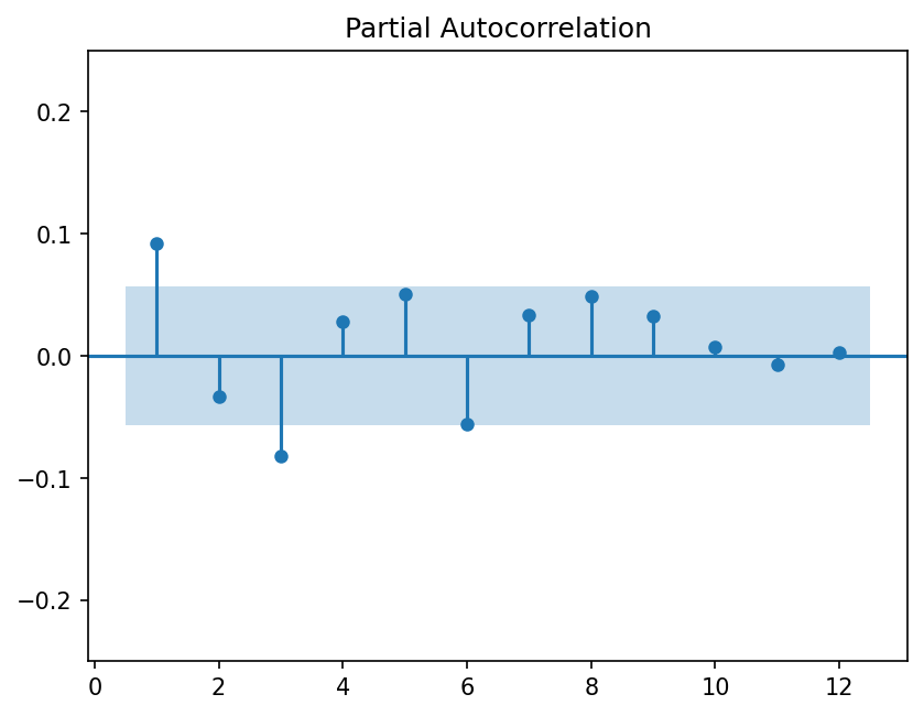
fig = sm.graphics.tsa.plot_pacf(vwret, lags=12, zero=False)
fig.axes[0].set_ylim(top=0.25, bottom=-0.25)

(-0.25, 0.25)

modsel = ar_select_order(vwret, maxlag=12, old_names=False)

modsel.bic

{(1,): -3556.6940863383184,
 0: -3553.820302624299,
 (1, 2, 3): -3551.593418073359,
 (1, 2): -3550.9120156201748,
 (1, 2, 3, 4): -3545.5448105552946,
 (1, 2, 3, 4, 5): -3541.5049850061137,
 (1, 2, 3, 4, 5, 6): -3538.088094282661,
 (1, 2, 3, 4, 5, 6, 7): -3532.2932200378154,
 (1, 2, 3, 4, 5, 6, 7, 8): -3528.0679679759337,
 (1, 2, 3, 4, 5, 6, 7, 8, 9): -3522.3229333570007,
 (1, 2, 3, 4, 5, 6, 7, 8, 9, 10): -3515.3199157587605,
 (1, 2, 3, 4, 5, 6, 7, 8, 9, 10, 11): -3508.3045433948228,
 (1, 2, 3, 4, 5, 6, 7, 8, 9, 10, 11, 12): -3501.244838723008}

vwret_ar1 = AutoReg(vwret, lags=1, old_names=False).fit()
print(vwret_ar1.summary())

                            AutoReg Model Results                             
==============================================================================
Dep. Variable:                 vwretd   No. Observations:                 1188
Model:                     AutoReg(1)   Log Likelihood                1805.381
Method:               Conditional MLE   S.D. of innovations              0.053
Date:                Mon, 06 Apr 2026   AIC                          -3604.763
Time:                        15:01:39   BIC                          -3589.525
Sample:                    02-28-1926   HQIC                         -3599.020
                         - 12-31-2024                                         
==============================================================================
                 coef    std err          z      P>|z|      [0.025      0.975]
------------------------------------------------------------------------------
const          0.0085      0.002      5.445      0.000       0.005       0.012
vwretd.L1      0.0923      0.029      3.191      0.001       0.036       0.149
                                    Roots                                    
=============================================================================
                  Real          Imaginary           Modulus         Frequency
-----------------------------------------------------------------------------
AR.1           10.8394           +0.0000j           10.8394            0.0000
-----------------------------------------------------------------------------

# testing for serial correlation in residuals

sm.stats.acorr_ljungbox(vwret_ar1.resid, lags=[3,6,9,12], return_df=True)

	lb_stat	lb_pvalue
3	9.749551	0.020820
6	17.014753	0.009229
9	21.864175	0.009320
12	22.474247	0.032536

modsel.aic

{(1, 2, 3, 4, 5, 6, 7, 8): -3573.6968351320606,
 (1, 2, 3, 4, 5, 6): -3573.5772131818712,
 (1, 2, 3, 4, 5, 6, 7, 8, 9): -3573.0216746415863,
 (1, 2, 3, 4, 5, 6, 7): -3572.852213065484,
 (1, 2, 3, 4, 5): -3571.924229776865,
 (1, 2, 3): -3571.872914587193,
 (1, 2, 3, 4, 5, 6, 7, 8, 9, 10): -3571.088531171805,
 (1, 2, 3, 4): -3570.8941811975874,
 (1, 2, 3, 4, 5, 6, 7, 8, 9, 10, 11): -3569.1430329363257,
 (1, 2, 3, 4, 5, 6, 7, 8, 9, 10, 11, 12): -3567.1532023929694,
 (1,): -3566.8338345952357,
 (1, 2): -3566.1216380055503,
 0: -3558.8901767527577}

vwret_ar8 = AutoReg(vwret, lags=8, old_names=False).fit()
print(vwret_ar8.summary())

                            AutoReg Model Results                             
==============================================================================
Dep. Variable:                 vwretd   No. Observations:                 1188
Model:                     AutoReg(8)   Log Likelihood                1803.623
Method:               Conditional MLE   S.D. of innovations              0.052
Date:                Mon, 06 Apr 2026   AIC                          -3587.247
Time:                        15:02:04   BIC                          -3536.514
Sample:                    09-30-1926   HQIC                         -3568.120
                         - 12-31-2024                                         
==============================================================================
                 coef    std err          z      P>|z|      [0.025      0.975]
------------------------------------------------------------------------------
const          0.0085      0.002      4.994      0.000       0.005       0.012
vwretd.L1      0.0959      0.029      3.297      0.001       0.039       0.153
vwretd.L2     -0.0183      0.029     -0.626      0.531      -0.076       0.039
vwretd.L3     -0.0908      0.029     -3.114      0.002      -0.148      -0.034
vwretd.L4      0.0249      0.029      0.852      0.394      -0.032       0.082
vwretd.L5      0.0613      0.029      2.098      0.036       0.004       0.119
vwretd.L6     -0.0579      0.029     -1.986      0.047      -0.115      -0.001
vwretd.L7      0.0291      0.029      0.996      0.319      -0.028       0.086
vwretd.L8      0.0491      0.029      1.690      0.091      -0.008       0.106
                                    Roots                                    
=============================================================================
                  Real          Imaginary           Modulus         Frequency
-----------------------------------------------------------------------------
AR.1            1.4255           -0.0000j            1.4255           -0.0000
AR.2            0.9871           -1.0260j            1.4238           -0.1281
AR.3            0.9871           +1.0260j            1.4238            0.1281
AR.4            0.0778           -1.3564j            1.3586           -0.2409
AR.5            0.0778           +1.3564j            1.3586            0.2409
AR.6           -1.1774           -0.8620j            1.4592           -0.3994
AR.7           -1.1774           +0.8620j            1.4592            0.3994
AR.8           -1.7923           -0.0000j            1.7923           -0.5000
-----------------------------------------------------------------------------

Now we can test the residuals for autocorrelation and whether they appear to come from a Normal distribution. In the first test, the null hypothesis is no autocorrelation; in the second it is normally-distributed data.

sm.stats.acorr_ljungbox(vwret_ar8.resid, lags=[3,6,9,12], return_df=True)

	lb_stat	lb_pvalue
3	0.009867	0.999740
6	0.098975	0.999981
9	1.814828	0.994069
12	1.967005	0.999455

vwret_ar8.test_normality()

Jarque-Bera    1993.004718
P-value           0.000000
Skewness          0.098459
Kurtosis          9.363718
dtype: float64

MA(q) models

As above, the MA(q) model is

\[r_t = \mu + \varepsilon_t + \theta_1 \varepsilon_{t-1} + \cdots + \theta_q \varepsilon_{t-q}.\]

Since the \(\varepsilon\) have zero mean, the expected value is given by

\[\E(r_t) = \mu.\]

The variance is

\[\begin{split} \begin{aligned} \var(r_t) &= \var(\varepsilon_t) + \var(\theta_1 \varepsilon_{t-1}) + \var(\theta_2 \varepsilon_{t-2}) + \cdots + \var(\theta_q \varepsilon_{t-q}) \\ &= \sigma^2_{\varepsilon} + \theta_1^2 \sigma^2_{\varepsilon} + \theta_2^2 \sigma^2_{\varepsilon} + \cdots + \theta_q^2 \sigma^2_{\varepsilon} \\ &= \sigma^2_{\varepsilon} \, (1 + \theta_1^2 + \theta_2^2 + \cdots + \theta_q^2). \end{aligned} \end{split}\]

In order to calculate the autocovariance, we’ll start with the simplest case: \(\gamma_1\) for an MA(1) model. First, notice that

\[r_t = \varepsilon_t + \theta_1 \varepsilon_{t-1}\]

implies that

\[r_{t-1} = \varepsilon_{t-1} + \theta_1 \varepsilon_{t-2}.\]

Therefore,

\[\begin{split} \begin{aligned} \cov(r_t, r_{t-1}) &= \cov(\varepsilon_t + \theta_1 \varepsilon_{t-1}, \;\varepsilon_{t-1} + \theta_1 \varepsilon_{t-2}) \\ &= \cov(\varepsilon_t,\varepsilon_{t-1}) + \cov(\varepsilon_t,\theta_1\varepsilon_{t-2}) + \cov(\theta_1\varepsilon_{t-1},\varepsilon_{t-1}) + \cov(\theta_1\varepsilon_{t-1}, \theta_1\varepsilon_{t-2}) \\ &= \theta_1 \sigma_{\varepsilon}^2, \end{aligned} \end{split}\]

where the last equality follows from the fact that \(\cov(r_t,r_{t-k}) = 0\) for all \(k\neq 0\).

Next let’s consider a model with one more lag:

\[\begin{split} \begin{aligned} r_t &= \varepsilon_t + \theta_1 \varepsilon_{t-1} + \theta_2 \varepsilon_{t-2}, \\ r_{t-1} &= \varepsilon_{t-1} + \theta_1 \varepsilon_{t-2} + \theta_2 \varepsilon_{t-3}. \end{aligned} \end{split}\]

In this case, we have

\[\begin{split} \begin{aligned} \cov(r_t, r_{t-1}) &= \cov(\varepsilon_t + \theta_1 \varepsilon_{t-1} + \theta_2 \varepsilon_{t-2},\; \varepsilon_{t-1} + \theta_1 \varepsilon_{t-2} + \theta_2 \varepsilon_{t-3}) \\ &= \cov(\theta_1 \varepsilon_{t-1}, \varepsilon_{t-1}) + \cov(\theta_2 \varepsilon_{t-2}, \theta_1 \varepsilon_{t-2}) \\ &= \theta_1 \sigma_{\varepsilon}^2 + \theta_1 \theta_2 \sigma_{\varepsilon}^2 \\ &= \theta_1 (1 + \theta_2)\, \sigma_{\varepsilon}^2. \end{aligned} \end{split}\]

Similarly, we can calculate \(\gamma_2\) as

\[\begin{split} \begin{aligned} \cov(r_t, r_{t-2}) &= \cov(\varepsilon_t + \theta_1 \varepsilon_{t-1} + \theta_2 \varepsilon_{t-2},\; \varepsilon_{t-2} + \theta_1 \varepsilon_{t-3} + \theta_2 \varepsilon_{t-4}) \\ &= \cov(\theta_2 \varepsilon_{t-2}, \varepsilon_{t-2}) \\ &= \theta_2 \sigma^2_{\varepsilon}. \end{aligned} \end{split}\]

Notice that any autocovariances of a higher order (i.e. \(\gamma_k\) when \(k>q\)) will be zero.

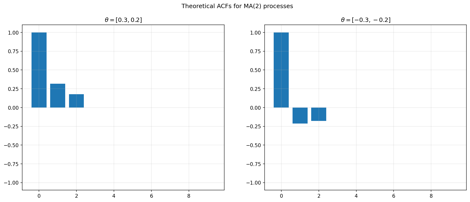
Generalizing the pattern from these examples, we can see that the autocovariance function for a MA(2) model is

\[\begin{split} \gamma_k = \begin{cases} \sigma^2_{\varepsilon} \sum_{j=0}^{q} \theta_j^2 & \text{if } k = 0, \\[1em] \sigma^2_{\varepsilon} \sum_{j=0}^{q-k} \theta_j \theta_{j+k} & \text{if } 1 \leq k \leq q, \\[1em] 0 & \text{if } k > q. \end{cases} \end{split}\]

For example, suppose \(\theta_1=0.3\) and \(\theta_2=0.2\). And for simplicity, let’s assume \(\mu=0\). Then

\[r_t = \varepsilon_t + 0.3 \varepsilon_{t-1} + 0.2 \varepsilon_{t-2}.\]

The variance is

\[\gamma_0 = 1^2 + 0.3^2 + 0.2^2 = 1.13.\]

We also have

\[\gamma_1 = 0.3 + 0.3\times 0.2 = 0.36\]

and

\[\gamma_2 = 0.2.\]

Therefore,

\[\begin{split} \begin{aligned} \rho(1) = \frac{0.36}{1.13} &= 0.3186 \\[1.5em] \rho(2) = \frac{0.2}{1.13} &= 0.1770. \end{aligned} \end{split}\]

θ = np.array([0.3, 0.2])

lags = 10

fig, (ax1, ax2) = plt.subplots(1,2,figsize=(16,6))

# MA(2) process
ma_coefs = np.r_[1, θ]
acf = arma_acf([1], ma_coefs, lags=lags)
ax1.bar(np.arange(lags), acf)
ax1.set_title(rf'$\theta={[float(x) for x in θ]}$')

# MA(2)
ma_coefs = np.r_[1, -θ]
acf = arma_acf([1], ma_coefs, lags=lags)
ax2.bar(np.arange(lags), acf)
ax2.set_title(rf'$\theta={[float(x) for x in -θ]}$')

for ax in (ax1, ax2):
    ax.set_ylim((-1.1,1.1))
    ax.grid(alpha=0.3)

fig.suptitle('Theoretical ACFs for MA(2) processes')
plt.show()

y = ArmaProcess(ma=ma_coefs).generate_sample(250)

fig, ax = plt.subplots(figsize=(10,4))
ax.plot(y, lw=1, marker='.', markersize=2)
plt.show()

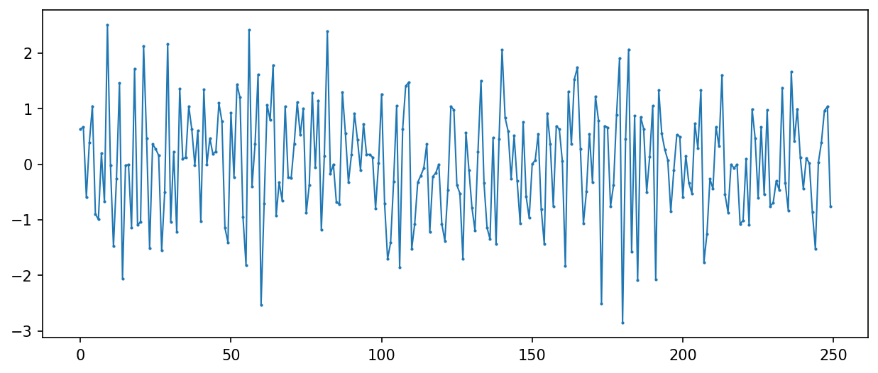
fig = sm.graphics.tsa.plot_acf(y, lags=12, zero=None)

vwret_ma9 = ARIMA(vwret, order=(0, 0, 9)).fit()

print(vwret_ma9.summary())

                               SARIMAX Results                                
==============================================================================
Dep. Variable:                 vwretd   No. Observations:                 1188
Model:                 ARIMA(0, 0, 9)   Log Likelihood                1818.875
Date:                Mon, 06 Apr 2026   AIC                          -3615.750
Time:                        15:05:08   BIC                          -3559.869
Sample:                    01-31-1926   HQIC                         -3594.690
                         - 12-31-2024                                         
Covariance Type:                  opg                                         
==============================================================================
                 coef    std err          z      P>|z|      [0.025      0.975]
------------------------------------------------------------------------------
const          0.0093      0.002      4.862      0.000       0.006       0.013
ma.L1          0.0944      0.019      5.097      0.000       0.058       0.131
ma.L2         -0.0087      0.021     -0.413      0.679      -0.050       0.033
ma.L3         -0.0932      0.022     -4.303      0.000      -0.136      -0.051
ma.L4          0.0078      0.023      0.346      0.729      -0.036       0.052
ma.L5          0.0740      0.023      3.281      0.001       0.030       0.118
ma.L6         -0.0277      0.021     -1.292      0.196      -0.070       0.014
ma.L7          0.0203      0.023      0.875      0.382      -0.025       0.066
ma.L8          0.0316      0.017      1.840      0.066      -0.002       0.065
ma.L9          0.0604      0.019      3.135      0.002       0.023       0.098
sigma2         0.0027   6.62e-05     41.370      0.000       0.003       0.003
===================================================================================
Ljung-Box (L1) (Q):                   0.00   Jarque-Bera (JB):              1917.60
Prob(Q):                              0.99   Prob(JB):                         0.00
Heteroskedasticity (H):               0.46   Skew:                             0.10
Prob(H) (two-sided):                  0.00   Kurtosis:                         9.22
===================================================================================

Warnings:
[1] Covariance matrix calculated using the outer product of gradients (complex-step).

vwret_ma9 = ARIMA(vwret, order=(0, 0, [1,3,5,9])).fit()
print(vwret_ma9.summary())

                                   SARIMAX Results                                   
=====================================================================================
Dep. Variable:                        vwretd   No. Observations:                 1188
Model:             ARIMA(0, 0, [1, 3, 5, 9])   Log Likelihood                1817.328
Date:                       Mon, 06 Apr 2026   AIC                          -3622.656
Time:                               15:05:17   BIC                          -3592.176
Sample:                           01-31-1926   HQIC                         -3611.169
                                - 12-31-2024                                         
Covariance Type:                         opg                                         
==============================================================================
                 coef    std err          z      P>|z|      [0.025      0.975]
------------------------------------------------------------------------------
const          0.0093      0.002      5.200      0.000       0.006       0.013
ma.L1          0.0990      0.018      5.413      0.000       0.063       0.135
ma.L3         -0.0998      0.021     -4.855      0.000      -0.140      -0.060
ma.L5          0.0779      0.022      3.550      0.000       0.035       0.121
ma.L9          0.0545      0.018      3.095      0.002       0.020       0.089
sigma2         0.0027   6.52e-05     42.138      0.000       0.003       0.003
===================================================================================
Ljung-Box (L1) (Q):                   0.02   Jarque-Bera (JB):              1836.61
Prob(Q):                              0.89   Prob(JB):                         0.00
Heteroskedasticity (H):               0.46   Skew:                             0.09
Prob(H) (two-sided):                  0.00   Kurtosis:                         9.09
===================================================================================

Warnings:
[1] Covariance matrix calculated using the outer product of gradients (complex-step).

ARMA(p,q) model

ARMA models combine properties of both AR and MA processes. They are particularly useful in modeling volatility.

vwret_arma = ARIMA(vwret, order=(1, 0, 2)).fit()
print(vwret_arma.summary())

                               SARIMAX Results                                
==============================================================================
Dep. Variable:                 vwretd   No. Observations:                 1188
Model:                 ARIMA(1, 0, 2)   Log Likelihood                1808.439
Date:                Mon, 06 Apr 2026   AIC                          -3606.878
Time:                        15:05:20   BIC                          -3581.478
Sample:                    01-31-1926   HQIC                         -3597.306
                         - 12-31-2024                                         
Covariance Type:                  opg                                         
==============================================================================
                 coef    std err          z      P>|z|      [0.025      0.975]
------------------------------------------------------------------------------
const          0.0093      0.002      5.487      0.000       0.006       0.013
ar.L1          0.5229      0.352      1.485      0.138      -0.167       1.213
ma.L1         -0.4340      0.355     -1.223      0.221      -1.129       0.261
ma.L2         -0.0784      0.027     -2.863      0.004      -0.132      -0.025
sigma2         0.0028   6.04e-05     46.125      0.000       0.003       0.003
===================================================================================
Ljung-Box (L1) (Q):                   0.02   Jarque-Bera (JB):              2254.04
Prob(Q):                              0.90   Prob(JB):                         0.00
Heteroskedasticity (H):               0.43   Skew:                             0.09
Prob(H) (two-sided):                  0.00   Kurtosis:                         9.75
===================================================================================

Warnings:
[1] Covariance matrix calculated using the outer product of gradients (complex-step).