U.S. market returns

import numpy as np
import pandas as pd
import matplotlib.pyplot as plt

import wrds

db = wrds.Connection()

Loading library list...
Done

Any data that we observe at regular intervals over time is a time series. An example could be stock prices or returns. For example, let’s look the S&P 500 index since 2000.

sp500 = db.get_table('crsp', 'dsp500', date_cols=['caldt'], columns=['caldt', 'spindx']).set_index('caldt')

sp500 = sp500.dropna().squeeze()

sp500 = sp500.loc['2000-01-01':]

Show code cell source

Hide code cell source

def ts_plot(ts):
    
    fig = plt.figure(figsize=(16, 9))

    # Set up axes
    width = 0.85
    height = 0.5
    space = 0.005

    rect_lvl  = [(1-width)+space, height+space, width, height]
    rect_ret   = [(1-width)+space, 0, width, height-space]
    rect_hist = [0, 0, 1-width, height-space]

    ax_ret = fig.add_axes(rect_ret)
    ax_lvl = fig.add_axes(rect_lvl, sharex=ax_ret)
    ax_hist = fig.add_axes(rect_hist, sharey=ax_ret)

    # Plot index level with moving average
    ts.plot(ax=ax_lvl, label='Index')
    ts.rolling(200).mean().plot(ax=ax_lvl, lw=3, label='200-day MA')

    # Plot return with rolling volatility
    ret = ts.pct_change()
    ret.plot(ax=ax_ret, label='Return')
    ret.rolling(21).std().plot(ax=ax_ret, lw=3, label='21-day volatility')

    # Plot return histogram
    ret.hist(bins=100, orientation='horizontal', ax=ax_hist, density=True)

    # Add pdf of normal distribution
    from scipy.stats import norm, gaussian_kde
    μ, σ = ret.mean(), ret.std()
    x = np.linspace(ret.quantile(0.005), ret.quantile(0.995), 100)
    pdf = norm.pdf(x, μ, σ)
    ax_hist.plot(pdf, x, 'k:', label='Normal PDF')

    # Kernel density estimation
    kde = gaussian_kde(ret.dropna())
    ax_hist.plot(kde.pdf(x), x, label='Estimated PDF')

    # Formatting
    ax_hist.legend(loc='upper left')
    ax_hist.grid(alpha=0.3)
    textstr = '$\\mu={:0.4f}$\n$\\sigma={:0.3f}$\nSkew=${:0.2f}$\nKurt=${:0.1f}$'
    ax_hist.text(0.05, 0.05, textstr.format(μ, σ, ret.skew(), ret.kurt()),
                 transform=ax_hist.transAxes, fontsize=10)
    ax_hist.invert_xaxis()
    
    ax_hist.tick_params(direction='in', left=True, right=True, bottom=False, labelbottom=False)
    ax_ret.tick_params(direction='in', left=True, right=True, top=True, labeltop=False, labelleft=False)
    ax_lvl.tick_params(direction='in', left=True, right=True, labelbottom=False)

    for ax in [ax_lvl, ax_ret]:
        ax.set_xlim((ts.index[0], ts.index[-1]))
        ax.grid(alpha=0.3)
        ax.set_xlabel('')
        ax.legend(loc='upper left', fontsize=14)

    plt.show()

ts_plot(sp500)

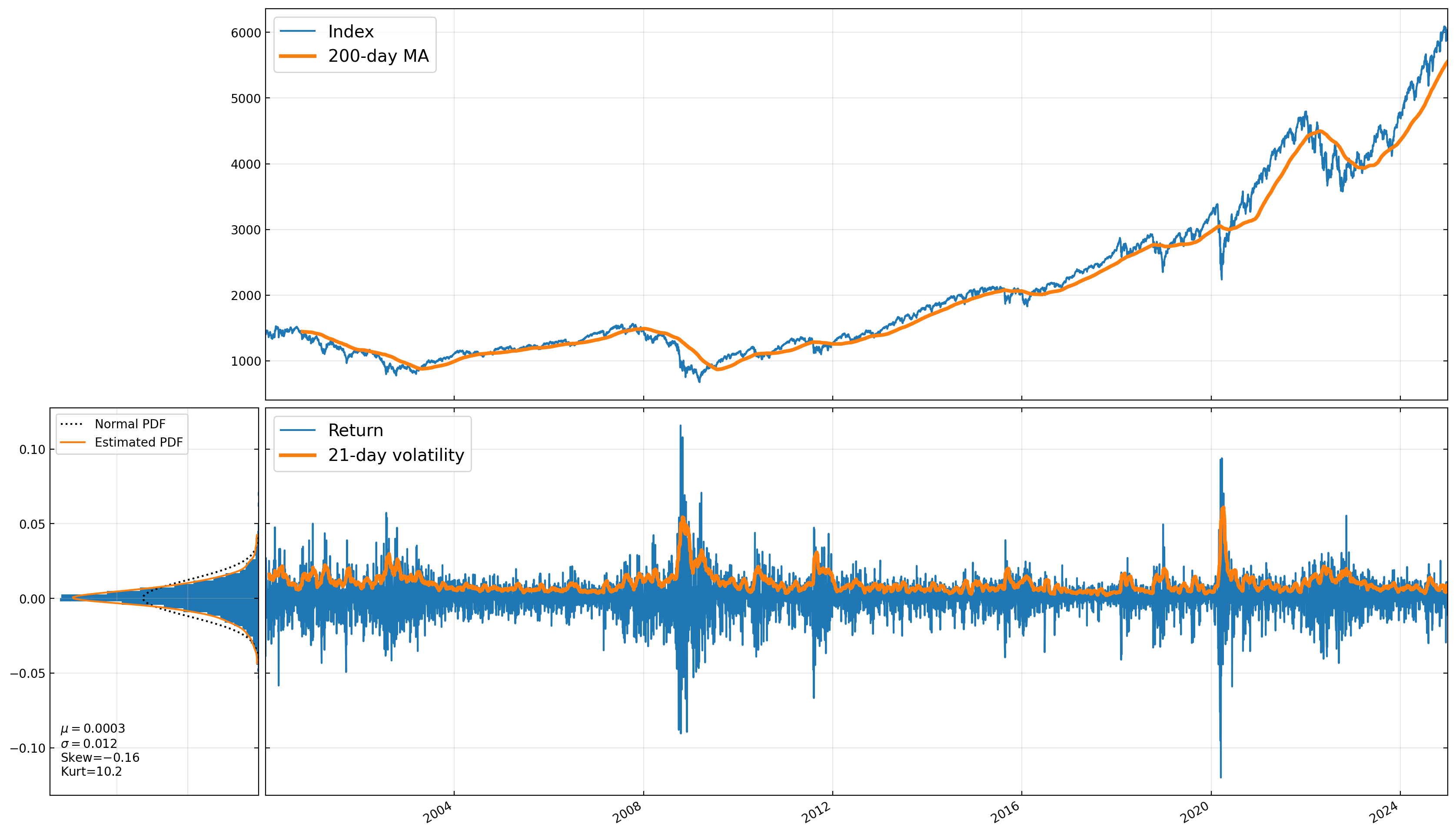
rets = sp500.pct_change().dropna()

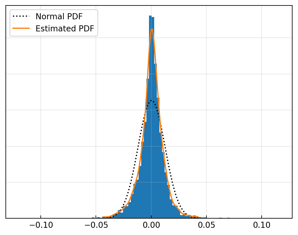
# Plot return histogram
ax = rets.hist(bins=100, density=True)

# Add pdf of normal distribution
from scipy.stats import norm, gaussian_kde
μ, σ = rets.mean(), rets.std()
x = np.linspace(rets.quantile(0.005), rets.quantile(0.995), 100)
pdf = norm.pdf(x, μ, σ)
ax.plot(x, pdf, 'k:', label='Normal PDF')

# Kernel density estimation
kde = gaussian_kde(rets.dropna())
ax.plot(x, kde.pdf(x), label='Estimated PDF')

ax.legend(loc='upper left')
ax.tick_params(direction='in', left=False, labelleft=False)
ax.grid(alpha=0.3)

plt.show()

rets.describe()

count      6288.0
mean     0.000297
std      0.012215
min     -0.119841
25%     -0.004793
50%      0.000597
75%      0.005928
max        0.1158
Name: spindx, dtype: Float64

rets.skew(), rets.kurt()

(-0.16201426750865283, 10.19031755909176)

There are several statistical tests we can use to test the null hypothesis that data are drawn from a normal distribution. Two that are available in scipy are due to D'agostino and Pearson [1973] and the Shapiro and Wilk [1965]. The former combines information about the skewness and kurtosis of a series; the latter is a more complicated test that uses information about order statistics.

Extra credit

To calculate the D’agostino and Pearson test statistic, we calculate the sample mean and standard deviation of the data,

\[ \bar{X} = \frac{1}{n} \sum_{i=1}^{n} X_i \]

\[ s = \sqrt{\frac{1}{n} \sum_{i=1}^{n} (X_i - \bar{X})^2}. \]

We then calculate the sample skewness and kurtosis:

\[ g_1 = \frac{ \frac{1}{n} \sum_{i=1}^{n} (X_i - \bar{X})^3 }{ s^3 } \]

\[ g_2 = \frac{ \frac{1}{n} \sum_{i=1}^{n} (X_i - \bar{X})^4 }{ s^4 } - 3 \]

Next, we make some statistical adjustments to make the skewness and kurtosis statistics normally distributed:

\[ Y_1 = g_1 \sqrt{ \frac{ (n+1)(n+3) }{6(n-2)} } \]

\[ \beta_2 = \frac{3(n^2 + 27n - 70)(n+1)(n+3)}{(n-2)(n+5)(n+7)(n+9)} \]

\[ W = \sqrt{ -1 + \sqrt{1 + 2(\beta_2 - 1)} } \]

The normalized statistics are then:

\[Z_1 = \frac{ Y_1 }{ \sqrt{ 1 + W } } \]

\[ Z_2 = \frac{ (g_2 + 3) - (3(n-1)/(n+1)) }{ \sqrt{ \frac{24n(n-2)(n-3)}{(n+1)^2(n+3)(n+5)} } } \]

Finally, we calculate the \(K^2\) statistic.

\[K^2 = Z_1^2 + Z_2^2.\]

This statistic has a \(\chi^2_{(2)}\) distribution under the null hypothesis that the \(X_i\) are drawn from a Normal distribution.

from scipy.stats import normaltest, shapiro

normaltest(rets)

NormaltestResult(statistic=1141.688127847064, pvalue=1.2177917029121804e-248)

shapiro(rets)

/var/folders/8b/3b5yf0214zvg3prfcqs6wx3c0000gq/T/ipykernel_62578/2132643539.py:1: UserWarning: scipy.stats.shapiro: For N > 5000, computed p-value may not be accurate. Current N is 6288.
  shapiro(rets)

ShapiroResult(statistic=0.9019364062429657, pvalue=4.684110917502552e-53)