Math background

We begin with a brief review of some basic mathematical facts that will be useful in the remainder of the course.

Show code cell source

Hide code cell source

import numpy as np
import pandas as pd
import matplotlib.pyplot as plt

plt.rcParams['figure.dpi'] = 200

# A helper function for plotting functions
def plot(func, xlim=(-3,3), *args):
    x = np.linspace(*xlim, 250)
    fig, ax = plt.subplots(figsize=(8,6))
    ax.plot(x, func(x), *args)
    ax.grid(alpha=0.25)

\(e\) and the exponential function

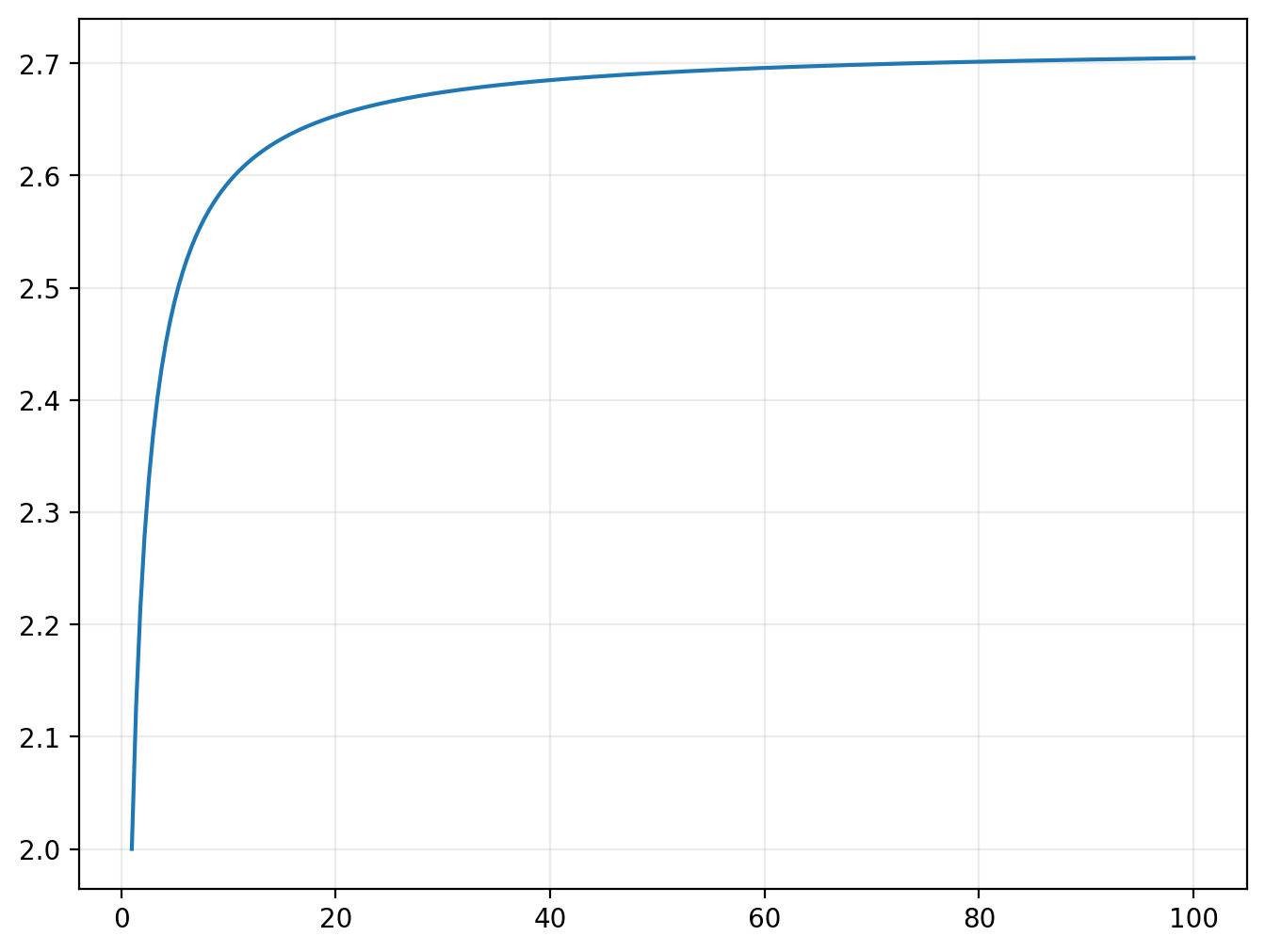
Consider the function

\[f(n) = \left(1+{\frac {1}{n}}\right)^{n},\]

plotted below with values of \(n\) ranging from 1 to 100. As \(n\) increases, it approaches a value of approximately 2.718.

plot(lambda n: (1+1/n)**n, (1,100))

Check your understanding

What is the purpose of the lambda function here? How else could we do the same thing?

The number \(e\) has a fascinating history, recounted in the excellent book e: The Story of a Number by Eli Maor.

This number is the irrational number \(e\), also called Euler’s number; it is defined as

\[ e := \lim _{n\to \infty }\left(1+{\frac {1}{n}}\right)^{n}. \]

More generally, the exponential function is defined as

\[\exp(x) := e^x = \lim _{n\to \infty }\left(1+{\frac {x}{n}}\right)^n.\]

Extra credit

You may be wondering why this isn’t written as

\[e^x = \lim _{n\to \infty }\left(1+{\frac {1}{n}}\right)^{nx}.\]

The two are equivalent. To see this, let \(k=\frac{n}{x}\). For a fixed value of \(x\), as \(n\to\infty\), \(k\to\infty\). So

\[\begin{equation*} \lim_{n\to \infty }\left(1+{\frac {x}{n}}\right)^n = \lim_{k\to \infty }\left(1+{\frac{1}{k}}\right)^{kx} = \left[\lim_{k\to \infty }\left(1+{\frac{1}{k}}\right)^{k}\right]^x = e^x. \end{equation*}\]

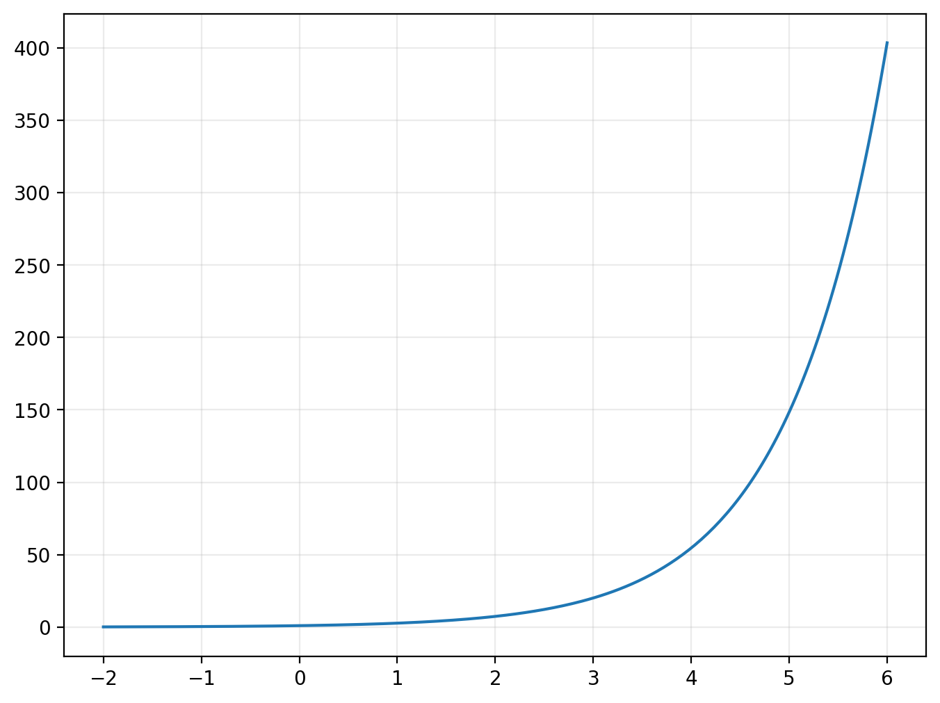
The exponential function plays a critical role in models of things that grow, be it bacteria in a culture or money in a bank account. As the figure below makes clear, the function gets large very quickly.

from numpy import exp

[exp(x) for x in [0, 1, 2]]

plot(exp, xlim=(-2,6))

Fun fact

If you want to impress your friends tell them that

\[e^{\pi i} + 1 = 0.\]

If you really want to impress them, prove it!

The inverse of the exponential function is the natural logarithm:

\[\ln(e^x) = x.\]

Economists just call the natural logarithm “log”; there is never a need to distinguish this from the logarithm in any other base.

While \(e^{\ln(10)}\) is obviously exactly equal to 10, note that the answer is represented with a tiny amount of error. This is due to the accuracy problems inherent in the floating-point system for representing real numbers. For all practical purposes in financial applications, errors this small will be irrelevant.

from numpy import log, pi as π

exp(log(10))

10.000000000000002

log(10)

2.302585092994046

plot(log, (0.005,25))

Logarithms have the property that

\[\ln(xy) = \ln(x) + \ln(y).\]

Factorials

The factorial of a positive integer \(n\) is the product of all integers from 1 up to \(n\):

\[{\displaystyle n!=n\cdot (n-1)\cdot (n-2)\cdot (n-3)\cdot \cdots \cdot 3\cdot 2\cdot 1\,.}\]

from scipy.special import factorial

factorial(5)

120.0

np.product(range(1,6))

120

Combinations

Factorials are critical for calculating the probabilities of possible outcomes. Given a set of \(n\) elements a combination is a choice of \(k\) items without regard to the ordering. There are \(_nC_k\) (“n-choose-k”) ways to select such a combination, where

\[_nC_k = \binom{n}{k} := \frac{n!}{k!(n-k)!}.\]

\(_nC_k\) is also referred to as the binomial coefficient.

For example, there are six ways we can choose two items from a set of four items:

from scipy.special import comb

comb(4,2)

6.0

Functions

A function is a mapping from an input to an output. For example,

(1)\[f(x) = 2x^2 - 3\]

is a function of the variable \(x\). Since \(x\) can take any real value and return a real value, we write \(f\!: \R \rightarrow \R\). (Actually, this particular \(f\) will also work on complex numbers, which we do not consider.)

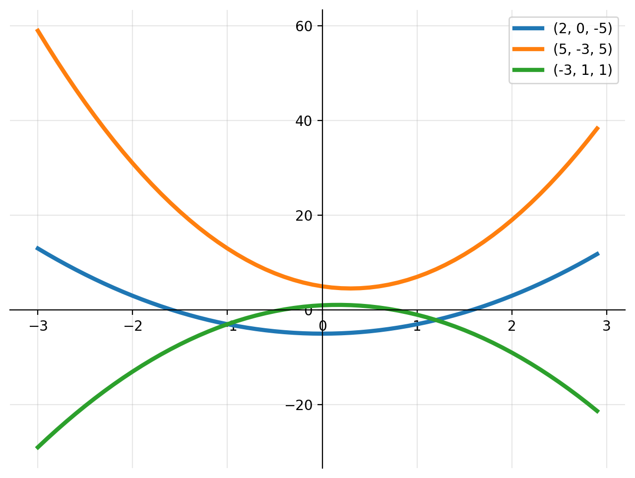
We might think of the function in (1) as a special case of a more general set of functions with parameters \(a\), \(b\), \(c\),

\[f(x; a, b, c) = ax^2 + bx + c.\]

The parameters — also called “coefficients” — are typically considered fixed, whereas \(x\) is a variable. The figure below shows three such functions, with different parameters \((a, b, c)\).

Show code cell source

Hide code cell source

def f(x, a, b, c):
    return a*x**2 + b*x + c

fig, ax = plt.subplots(figsize=(8,6))

# Set up the spines
for loc in ['right', 'top']:
    ax.spines[loc].set_color('none')
for loc in ['bottom', 'left']:
    ax.spines[loc].set_position(('data',0))
ax.xaxis.set_ticks_position('bottom')
ax.yaxis.set_ticks_position('left')

x = np.arange(-3, 3, 0.1)
for params in [(2,0,-5), (5,-3,5), (-3,1,1)]:
    ax.plot(x, f(x, *params), label=str(params), lw=3)

ax.legend(loc='upper right')
ax.grid(alpha=0.3)
plt.show()

The fundamental theorems of calculus

Let \(f\) be a continuous function defined on the closed interval \([a,b]\). Let \(F\) be the function defined as

\[F(x) = \int_a^x f(z) \, dz.\]

Then \(F\) is differentiable on the open interval \((a,b)\) and

\[F'(x) = f(x)\]

for all \(x\) in \((a,b)\). Moreover,

\[\int_a^b f(x) \, dx = F(b) - F(a).\]

That is, the area under the curve \(f(x)\) from points \(a\) to \(b\) is the difference in the integral evaluated at those points.

The Gaussian integral

Consider the function

\[f(z) = e^{-z^2},\]

plotted below:

plot(lambda z: np.exp(-z**2), xlim=(-4,4))

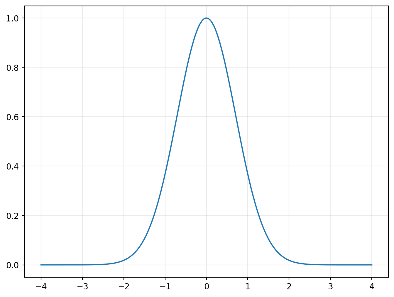
Somewhat incredibly, the area under this curve — called the Gaussian integral, named for Carl Friedrich Gauss — is \(\sqrt{\pi}\):

(2)\[ \int _{-\infty }^{\infty }e^{-z^2}\,dz = \sqrt{\pi}. \]

We can confirm using the sympy package for doing symbolic math.

import sympy as sp
from sympy import oo  # infinity symbol

z = sp.symbols('z')

# Calculate the Gaussian integral
x = sp.integrate(sp.exp(-z**2), (z, -oo, oo))

print("x is:", x)

x is: sqrt(pi)

# renders as a mathematical object in Jupyter Notebooks
x

\[\displaystyle \sqrt{\pi}\]

For a more general form of the integral, use the change of variables

\[z = \frac{x-b}{\sqrt{2c^2}},\]

where \(b\) and \(c\) are constants, implying that

\[dz = \frac{dx}{\sqrt{2c^2}}.\]

Then

\[\begin{equation*} {\large\int_{-\infty }^{\infty }} e^{-z^2}\,dz \; = \; \frac{1}{\sqrt{2c^2}} {\large\int_{-\infty }^{\infty }}\exp\left\{-\frac{1}{2}\left(\frac{x-b}{c}\right)^2\right\}dx, \end{equation*}\]

so

\[{\large\int_{-\infty }^{\infty }}\exp\left\{-\frac{1}{2}\left(\frac{x-b}{c}\right)^2\right\}dx = \sqrt{2 \pi c^2}.\]

We will revisit this fact when we discuss the normal probability distribution.

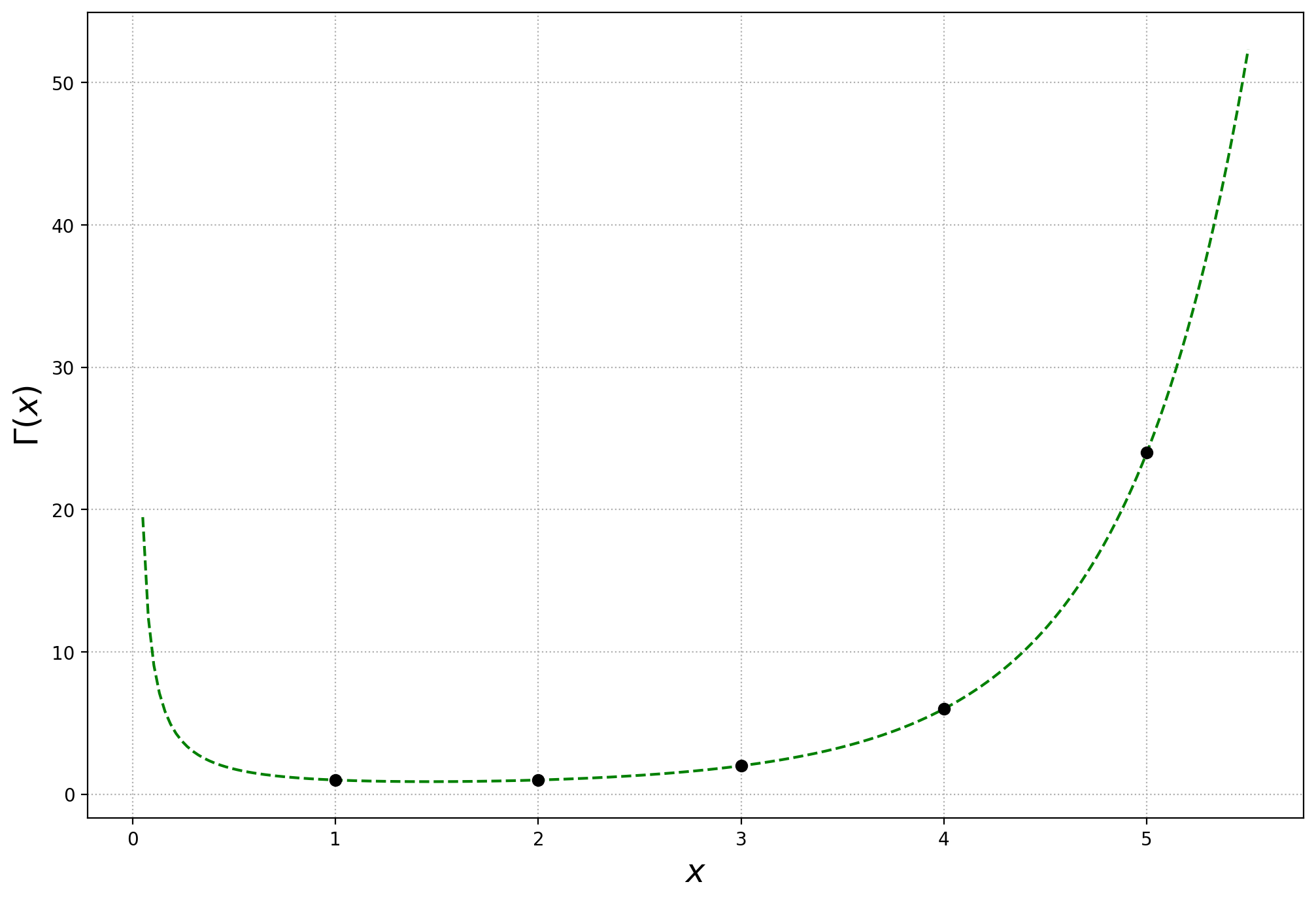
The gamma function

The gamma function,

\[\Gamma(x) := \int _{0}^{\infty }s^{x-1}e^{-s}ds, \quad x>0,\]

is a generalization of the factorial. That is, for any positive integer \(n\),

\[\Gamma(n+1) = n\Gamma(n) = n!\]

But \(\Gamma(x)\) is defined over any positive real number, not just the integers. It is effectively a continuous function that connects the values of the factorial function, as shown below.

Show code cell source

Hide code cell source

from scipy.special import gamma

plt.figure(figsize=(12,8))

z = np.linspace(0.05,5.5,200)
plt.plot(z, gamma(z), 'g--')

n = np.arange(6)
plt.plot(n, gamma(n), 'ko')

plt.xlabel('$x$', fontsize=18)
plt.ylabel(r'$\Gamma(x)$', fontsize=18)
plt.grid(ls=':')
plt.show()

Another useful fact about the gamma function is that

\[\Gamma\left(\frac{1}{2}\right) = \sqrt{\pi}.\]

Extra credit

This can be seen by writing the Gaussian integral (2) as

\[\sqrt{\pi} = \int _{-\infty }^{\infty }e^{-z^{2}}dz=2\int _{0}^{\infty }e^{-z^{2}}dz.\]

The second equality follows from the fact that \(e^{-z^2}\) is an even function, meaning it is symmetric about zero — that is, \(f(x)=f(-x)\).

After the change of variable \(z=\sqrt{s}\),

\[2\int _{0}^{\infty}e^{-z^2}dz = 2\int_{0}^{\infty}\frac{1}{2}\ e^{-s}\ s^{-\frac{1}{2}}ds = \int_{0}^{\infty}e^{-s}\ s^{-\frac{1}{2}}ds = \Gamma \left({\frac {1}{2}}\right).\]

Exercise

Using the gamma function defined in scipy.special, write a loop that that confirms that

\[\Gamma(n+1) = n\Gamma(n)\]

for \(n\in\{1,2,\ldots,5\}\).

Solution

from scipy.special import gamma as Γ

for n in range(1,6):
    assert n*Γ(n) == Γ(n+1)

Taylor series

The Taylor series approximation of a function, \(f(x)\), around some point \(a\) is

\[f(x) = f(a) + f'(a)(x-a) + \frac{f''(a)}{2!}(x-a)^{2} + \frac{f'''(a)}{3!}(x-a)^{3} + \cdots\]

where \(f'\) is the first derivative, \(f''\) is the second derivative, etc.

As we add more terms to the expansion, we will get arbitrarily close to the true function \(f(x)\) as long as we stay near \(a\). For example, let

\[f(x) = \ln(1+x),\]

and take the expansion around \(a=0\),

\[\begin{align*} \ln(1+x) &= \ln(1+a) + (1+a)^{-1}(x-a) - \frac{(1+a)^{-2}}{2}(x-a)^2 + \frac{2(1+a)^{-3}}{6}(x-a)^3 \cdots \\ &= 0 + x - \frac{1}{2}x^2 + \frac{1}{3}x^3 - \frac{1}{4}x^4 + \cdots \\ &= \sum_{k=1}^{\infty} \frac{(-1)^{k-1} x^k}{k}. \end{align*}\]

Key fact

If we keep only the first term of the expansion, we get a very useful fact about the logarithm function, namely that, when \(x\) is close to zero,

\[\ln(1+x) \approx x.\]

As the table below shows, the approximation is quite close for small numbers, but starts to degrade when \(x>0.1.\)

x	log(1+x)	Error	% Error
0.001000	0.001000	-0.000000	-0.05%
0.003981	0.003973	-0.000008	-0.20%
0.015849	0.015725	-0.000124	-0.79%
0.063096	0.061185	-0.001911	-3.12%
0.251189	0.224094	-0.027095	-12.09%
1.000000	0.693147	-0.306853	-44.27%

Including higher-order terms improves the approximation, as shown here:

Show code cell source

Hide code cell source

def plot_taylor_ln1px(n):
    '''Plot the Taylor series expansion of ln(1+x) near 0'''
    fig, ax = plt.subplots(figsize=(8,6))
    ax.set_xlim(-1.5,1.5)
    ax.set_ylim(-4,2)
    # Set up the spines
    for loc in ['right', 'top']:
        ax.spines[loc].set_color('none')
    for loc in ['bottom', 'left']:
        ax.spines[loc].set_position(('data',0))
    ax.xaxis.set_ticks_position('bottom')
    ax.yaxis.set_ticks_position('left')

    x = np.arange(-1.5, 1.5, 0.001)
    
    # Draw f(x) over x > -1
    fx = np.log(x[x>-1]+1)
    ax.plot(x[x>-1], fx, '-', color='r', lw=3)

    # Draw the Taylor approximation
    approx = 0
    for k in range(1,n+1):
        approx += (-1)**(k-1) * (1/k) * x**k
        
    ax.plot(x, approx, 'k--', lw=3)
    ax.text(-1, 1, f'N={n}', fontsize=18)

plot_taylor_ln1px(1)

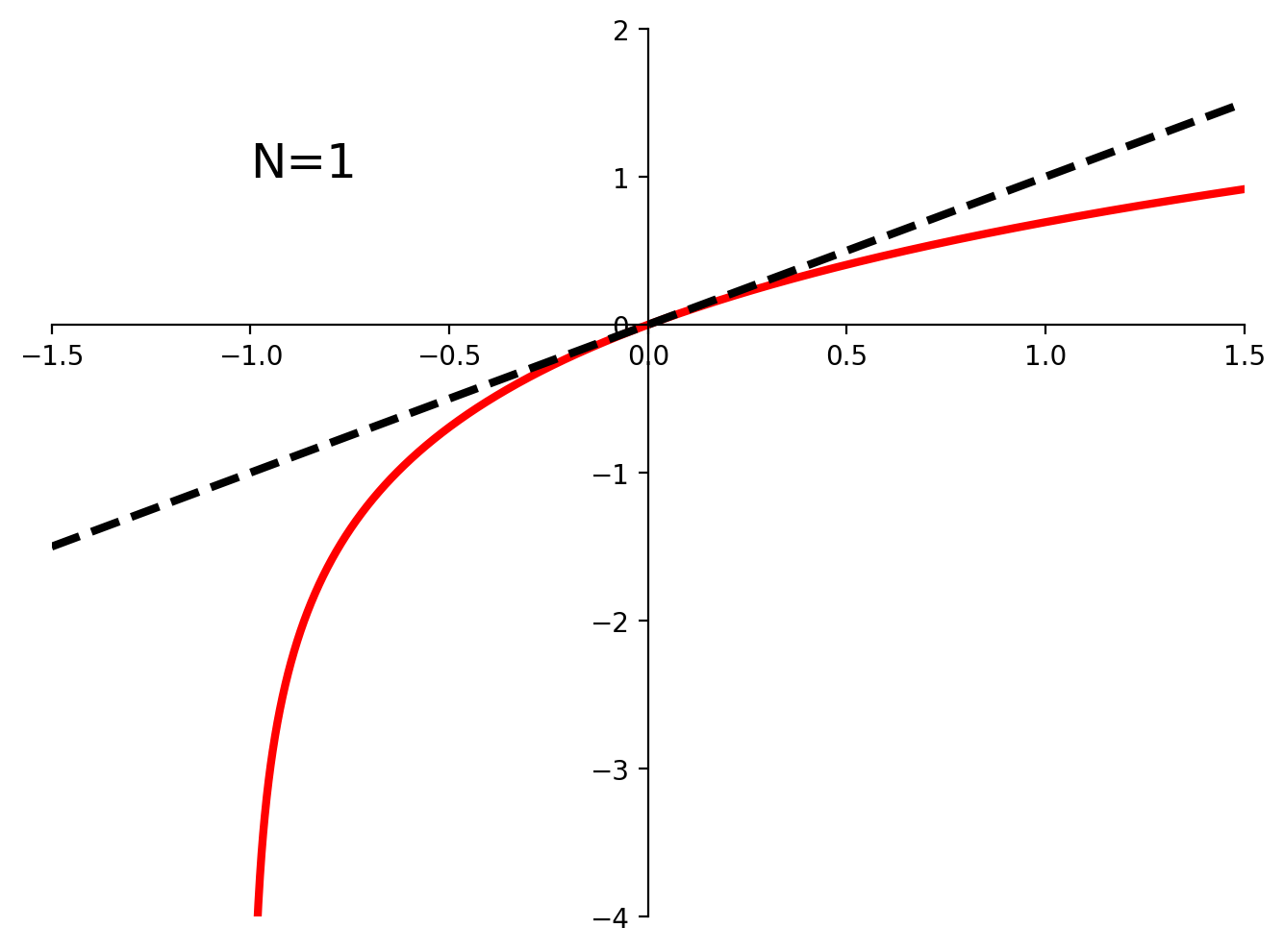
plot_taylor_ln1px(10)

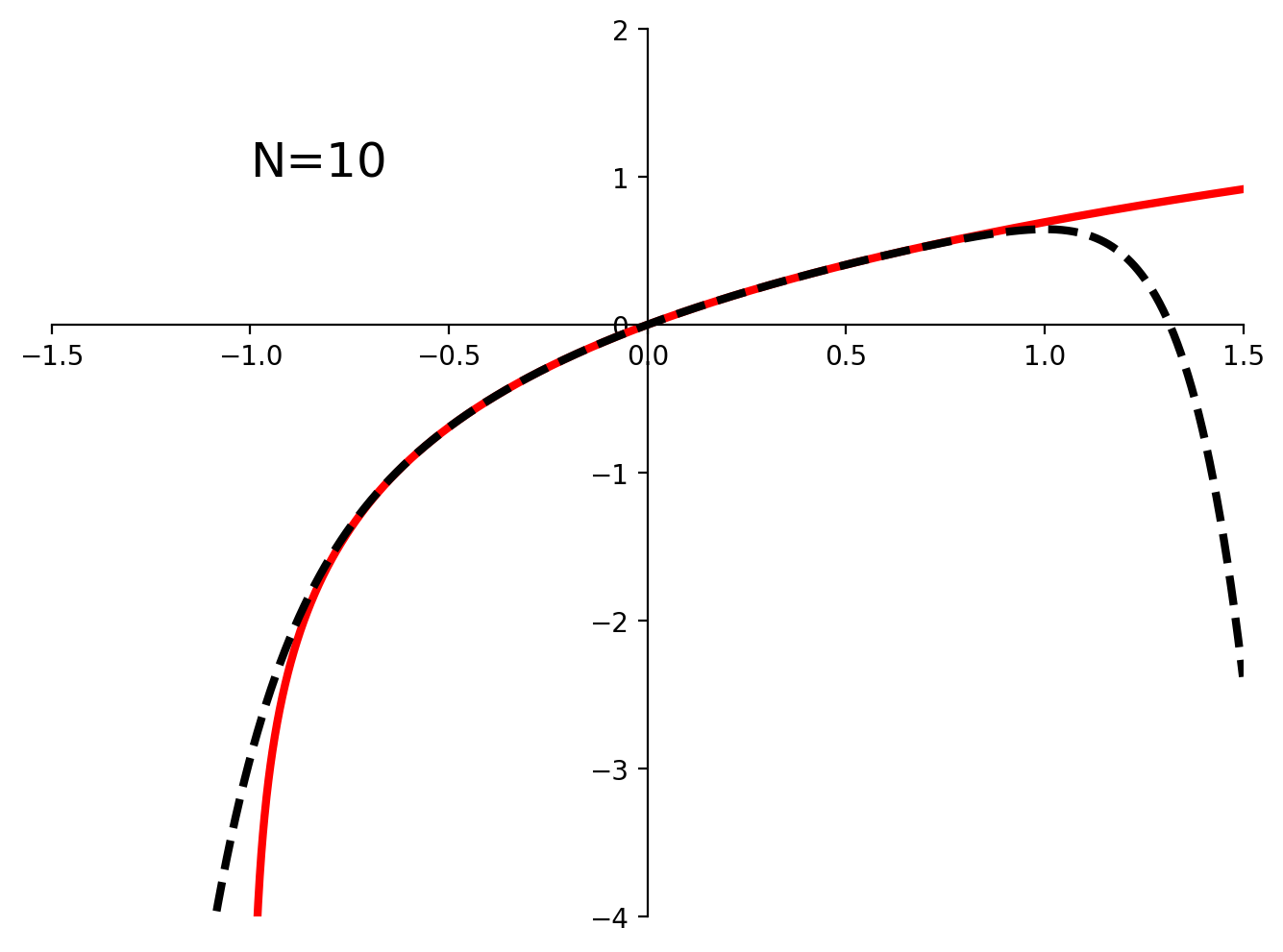
Notice that as we increase the number of terms in the polynomial the approximation (black dotted line) stays closer to the true function (red) for a wider range of values.

Exercise

Find the Taylor series expansion of \(e^x\) around \(x_0=0\). Write out the first four terms.

Solution

Since the derivative of \(e^x\) is also \(e^x\), we have \(f(0) = 1\), \(f'(0)=1\), and so on for all derivatives. The series therefore simplifies to

\[e^x = 1 + x + \frac{x^2}{2} + \frac{x^3}{3!} + \frac{x^4}{4!} + \cdots = \sum_{k=1}^{\infty} \frac{x^k}{k!}.\]

Sympy can also solve this problem:

x = sp.symbols('x')
f = sp.exp(x)
f.series(x, 0, 5)

\[ 1 + x + \frac{x^{2}}{2} + \frac{x^{3}}{6} + \frac{x^{4}}{24} + O\left(x^{5}\right) \]

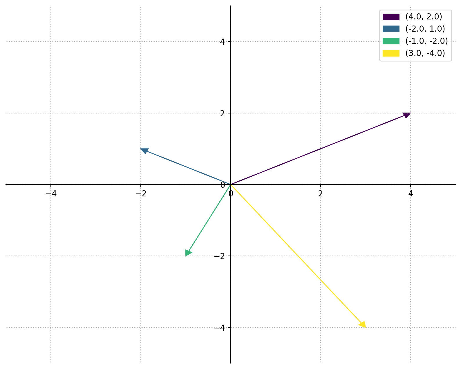
Vectors

A (Euclidean) vector is is a geometric object with direction and length.

For example, the vector (4,2) originates at the origin (0,0) and ends at the point (4,2).

a = np.array([4,2])
b = np.array([-2,1])
c = np.array([-1,-2])
d = np.array([3,-4])

Show code cell source

Hide code cell source

def plot_vectors(vecs, lims):
    '''A function for plotting vectors'''
    from matplotlib import cm
    
    fig, ax = plt.subplots(figsize=(10, 8))

    # Set the axes through the origin
    for spine in ['left', 'bottom']:
        ax.spines[spine].set_position('zero')
    for spine in ['right', 'top']:
        ax.spines[spine].set_color('none')

    ax.set(xlim=lims, ylim=lims)
    ax.grid(ls=':')

    # draw vectors
    colors = cm.viridis(np.linspace(0,1,len(vecs)))
    
    for v,c in zip(vecs,colors):
        v = v.flatten()
        ax.arrow(0, 0, *v,
                 head_width=0.15, head_length=0.15,
                 length_includes_head=True,
                 fc=c, ec=c,
                 label='({:.1f}, {:.1f})'.format(*v))
    plt.legend()
    plt.show()

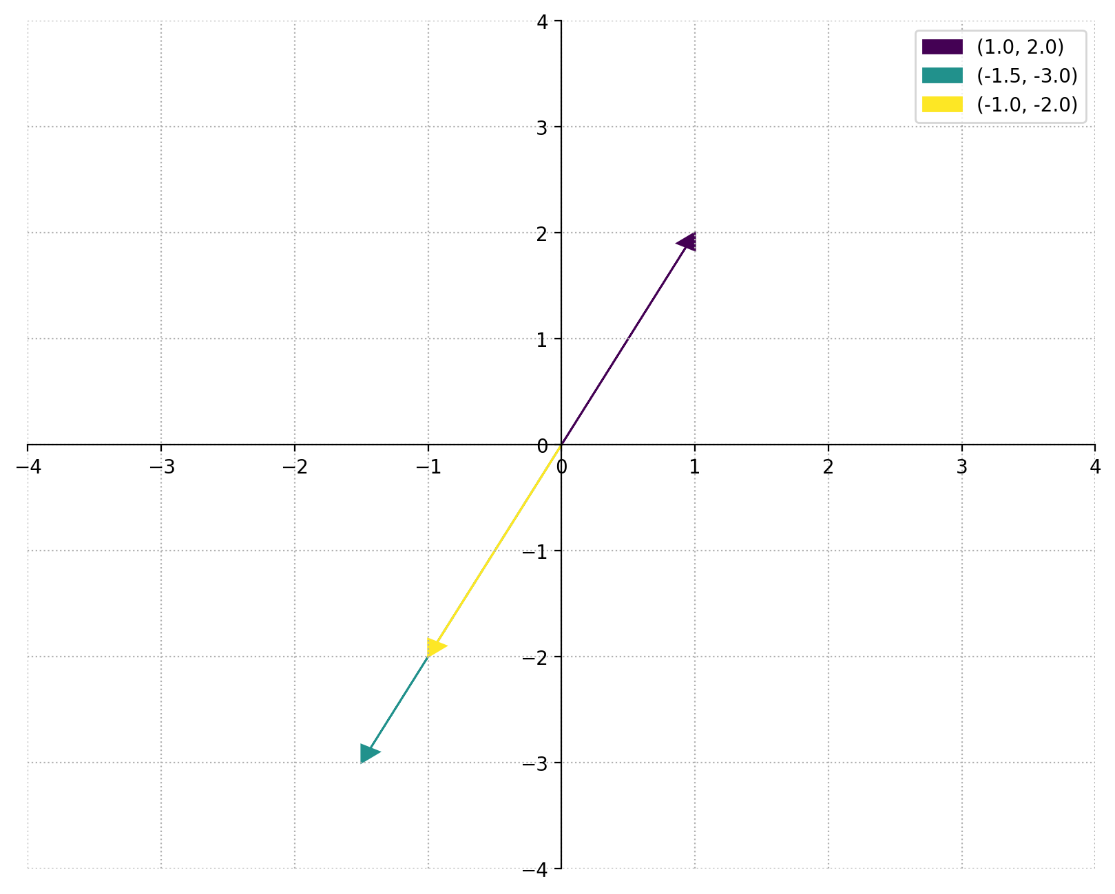
plot_vectors([a,b,c,d], (-5,5))

plot_vectors([-1*c, 1.5*c, c], (-4,4))

Vector norms

The length of a vector is the distance from the origin to the terminal point of the vector. It is given by the \(\ell^2\) or “Euclidean” norm

(3)\[||{\boldsymbol {x}}||_2 := \sqrt{\mathbf{x}\cdot\mathbf{x}} = \sqrt{x_{1}^{2}+\cdots +x_{n}^{2}}.\]

It is easy to see why this is true for vectors on a 2-dimensional plane if we remember the Pythagorean Theorem.

from numpy.linalg import norm

norm([3, -4])

5.0

plot_vectors([np.array([3,-4])], (-4,4))

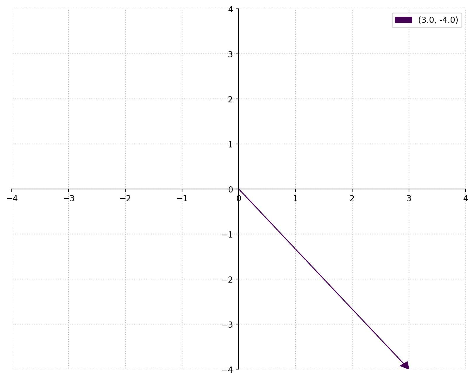
This is the distance between the origin and the point \((3,-4)\), which, by the Pythagorean theorm, is \(5\). The function works just as easily in higher dimensions:

norm([1, 1, 1])

1.7320508075688772

That is, the Euclidean distance between the origin and the point \((1,1,1)\) is \(\sqrt{3} \approx 1.73\).

The \(\ell^1\) norm is also known as the “Manhattan” norm or the “taxicab” norm because it measures the distance that a car would have to travel between two points on a road laid out on a grid as in New York City.

Other measures of distance, or norms, are possible. The \(\ell^1\) norm, for example, is given by

\[||{\boldsymbol {x}}||_1 := \sum _{i=1}^{n}\left|x_{i}\right|.\]

# l1 norm
norm([3, -4], ord=1)

7.0

Dot product

The expression under the square root in equation (3) is the dot product, \(\mathbf{x}\cdot \mathbf{x}\), where

\[\mathbf{a}\cdot \mathbf{b} := \sum_{i=1}^n a_i b_i = a_1b_1 + \ldots + a_nb_n.\]

There are several ways to calculate dot products in numpy, as shown below.

a

array([4, 2])

a.dot(a)

20

np.dot(a,a)

20

# Preferred method
a @ a

20

# calculate length of a
np.sqrt(a  @ a)

4.47213595499958

# equivalently
norm(a)

4.47213595499958

Angle between vectors

The angle \(\theta\) between two vectors follows

\[\cos(\theta) = \frac{a\cdot b}{||a||\cdot||b||},\]

so

\[\theta = \cos^{-1}\left(\frac{a\cdot b}{||a||\cdot||b||}\right).\]

Two vectors are orthogonal if the angle between them is \(\frac{\pi}{2}\) radians. Since \(\cos(\pi/2)=0\), vectors are orthogonal if and only if their dot product is zero.

# angle between a and b (in radians)
np.arccos( a.dot(b) / norm(a) / norm(b))

2.214297435588181

# convert to degrees
np.degrees(2.214297435588181)

126.86989764584402

# angle between b and c
np.arccos( b.dot(c) / norm(b) / norm(c))

1.5707963267948966

This is indeed equal to \(\pi/2\):

π/2

1.5707963267948966

So \(b\) and \(c\) must be orthoganal, which we may confirm by checking that their dot product is zero:

b @ c

0

In financial applications we often use the dot product of vectors to calculated a weighted sum. For example, suppose we have a vector of weights

\[\mathbf{w} = (w_1, w_2, w_3).\]

Then the dot product

\[\mathbf{x}\cdot\mathbf{w} = w_1 x_1 + w_2 x_2 + w_3 x_3\]

is simply the weighted sum of the elements of \(\mathbf{x}\).

Matrices

A matrix is a tabular collection of vectors, each with the same number of elements. For example, let \(\mathbf{A}\) be an \(m\times n\) matrix and \(\mathbf{B}\) be an \(n\times p\) matrix,

\[\begin{split}\mathbf {A} ={\begin{pmatrix}a_{11}&a_{12}&\cdots &a_{1n}\\a_{21}&a_{22}&\cdots &a_{2n}\\\vdots &\vdots &\ddots &\vdots \\a_{m1}&a_{m2}&\cdots &a_{mn}\\\end{pmatrix}},\quad \mathbf {B} ={\begin{pmatrix}b_{11}&b_{12}&\cdots &b_{1p}\\b_{21}&b_{22}&\cdots &b_{2p}\\\vdots &\vdots &\ddots &\vdots \\b_{n1}&b_{n2}&\cdots &b_{np}\\\end{pmatrix}}.\end{split}\]

Having defined matrices, it becomes useful to distinguish between two types of vectors: a \(1\times n\) row vector

\[{\displaystyle \mathbf{a} = (a_1, \ldots, a_n)},\]

and an \(n\times 1\) column vector

\[\begin{split}\mathbf{b} = \begin{pmatrix} b_1\\ \vdots\\ b_n \end{pmatrix}.\end{split}\]

We can think of a matrix either as a group of row vectors stack on top of each other, or a group of column vectors stacked next to each other.

Matrix multiplication

The matrix product \(\mathbf{C} = \mathbf{AB}\) is defined to be the \(m \times p\) matrix

\[\begin{split}{\displaystyle \mathbf {C} ={\begin{pmatrix}c_{11}&c_{12}&\cdots &c_{1p}\\c_{21}&c_{22}&\cdots &c_{2p}\\\vdots &\vdots &\ddots &\vdots \\c_{m1}&c_{m2}&\cdots &c_{mp}\\\end{pmatrix}}}\end{split}\]

such that

\[\begin{align*} c_{ij} &= a_{i1}b_{1j}+a_{i2}b_{2j}+\cdots +a_{in}b_{nj} \\ &= \sum_{k=1}^{n}a_{ik}b_{kj}, \end{align*}\]

for \(i=1,\ldots,m\) and \(j=1,\ldots,p.\) Obviously, such multiplication is only possible when the number of columns of \(\mathbf{A}\) equals the number of rows of \(\mathbf{B}.\)

The diagram below provides an illustration of the mechanics of matrix multiplication.

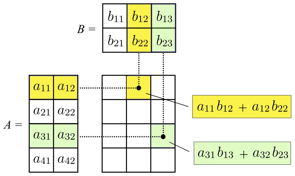
Fig. 1 Matrix multiplication. Source: Svjo, CC BY-SA 4.0, via Wikimedia Commons.

A matrix in numpy is just an array with two dimensions. Here we create two matrices, \(A\) and \(B\), to work with.

A = np.array([[ 3,  2, -2],
              [ 1, -4,  3],
              [-2,  1, -2]])

B = np.array([[ 1,  3, -2],
              [ 2,  -1,  2],
              [ 3,  1, -1]])

To multiply matrices we take the dot product.

A @ B

array([[  1,   5,   0],
       [  2,  10, -13],
       [ -6,  -9,   8]])

Identity matrix

The identity matrix has ones along the main diagonal and zeros elsewhere:

\[\begin{split}\mathbf{I} := {\begin{pmatrix}1 & 0 & \cdots & 0\\ 0 & 1 & \cdots & 0\\\vdots &\vdots &\ddots &\vdots \\0 & 0 & \cdots &1\\\end{pmatrix}}.\end{split}\]

Multiplying any matrix or vector by the appropriately-sized identity matrix is like multiplying any number by one — we just get the initial matrix or vector as the answer.

numpy follows a convention from other programs of using a pun to refer to the identity matrix — np.eye. Get it?

np.eye(3)

array([[1., 0., 0.],
       [0., 1., 0.],
       [0., 0., 1.]])

# multiply by the identity matrix
A @ np.eye(3)

array([[ 3.,  2., -2.],
       [ 1., -4.,  3.],
       [-2.,  1., -2.]])

Transpose

Two transformations of matrices are frequently used. The first is the transpose, in which all of the elements are reflected across the main diagonal. Equivalently, we can think of writing all of the rows as the columns, and all the columns as rows.

\[\begin{split}\mathbf{A}' := {\begin{pmatrix}a_{11}&a_{21}&\cdots &a_{m1}\\a_{12}&a_{22}&\cdots &a_{m2}\\\vdots &\vdots &\ddots &\vdots \\a_{1m}&a_{2m}&\cdots &a_{mn}\\\end{pmatrix}}\end{split}\]

A.T

array([[ 3,  1, -2],
       [ 2, -4,  1],
       [-2,  3, -2]])

The transpose of a row vector is a column vector, and vice versa. Therefore, the dot product \(\mathbf{x} \cdot \mathbf{x}\) for a column vector \(\mathbf{x}\) can also be written as \(\mathbf{x}'\mathbf{x}\).

Warning

If \(\mathbf{x}\) were a row vector, \(\mathbf{x}'\mathbf{x}\) would be a square matrix, not a scalar. Always pay attention to the dimensions of what is being multiplied.

For example, given a vector of portfolio weights

\[\boldsymbol{\omega} = (\omega_1, \ldots, \omega_N)'\]

with corresponding asset returns

\[\mathbf{R} = (R_1, \ldots, R_N)',\]

the portfolio return is simply \(\boldsymbol{\omega}' \mathbf{R}\).

Another often-seen example is defining an \(N\)-vector of ones,

\[\mathbf{1} = (1, 1, \ldots, 1)'\]

in which case

\[\mathbf{1}'\mathbf{1} = N.\]

Note

The transpose is sometimes written as \(\mathbf{x}^\intercal\), but in economics and finance, people mostly use the “prime” symbol as in \(\mathbf{x}'\) instead. While this could be confused with the derivative symbol, the meaning should usually be quite clear. For example, while it is reasonable to assume that \(f'(x)\) is the derivative of the function \(f\) with respect to \(x\), it wouldn’t make sense that \(\mathbf{x}'\) would be a derivative since \(\mathbf{x}\) isn’t a function.

Inverse

The second important transformation is the inverse of \(\mathbf{A}\). This is the matrix \(\mathbf{A}^{-1}\) such that

\[\mathbf{A} \times \mathbf{A}^{-1} = \mathbf{I}.\]

If a matrix is not square it may have a left inverse and a right inverse. A square matrix has only one inverse, which can be multiplied on either side.

from numpy.linalg import inv

A @ inv(A)

array([[ 1.00000000e+00,  0.00000000e+00,  0.00000000e+00],
       [ 0.00000000e+00,  1.00000000e+00, -4.44089210e-16],
       [-1.11022302e-16,  0.00000000e+00,  1.00000000e+00]])

There is some rounding error in this calculation, but if you look closely you’ll see that this is indeed the identity matrix. We can see this by using np.allclose(a,b), a boolean function that returns True when the corresponding elements of a and b are all “close,” meaning the difference between them is negligible, perhaps due to numerical imprecision.

np.allclose(A @ inv(A), np.eye(3))

True

In the case of a \(2\times 2\) matrix, the inverse is given by

(4)\[\begin{split} \left(\begin{array}{ll} a & b \\ c & d \end{array}\right)^{-1}=\frac{1}{a d-c b}\left(\begin{array}{cc} d & -b \\ -c & a \end{array}\right) \end{split}\]

Exercise

Show that equation (4) is correct by multiplying the inverse by the original matrix and confirming that the result is the identity matrix.

Solving systems of equations

Matrices are especially useful for compactly writing systems of equations. For example, consider the system of \(m\) linear equations

\[\begin{split}{\begin{matrix}a_{11}x_{1}+\cdots +a_{1n}x_{n}=b_{1}\\a_{21}x_{1}+\cdots +a_{2n}x_{n}=b_{2}\\\vdots \\a_{m1}x_{1}+\cdots +a_{mn}x_{n}=b_{m}\end{matrix}}.\end{split}\]

By defining the column vectors \(\mathbf{x}\) and \(\mathbf{b}\), the system can be written in matrix notation as \({\displaystyle \mathbf {Ax} =\mathbf {b}}.\)

Premultiplying both sides of this equation by \(\mathbf{A}^{-1}\) allows us to solve for \(\mathbf{x}\),

\[\mathbf{x} = \mathbf{A}^{-1} \mathbf{b}.\]

For example, suppose we wish to solve the system of equations

\[\begin{align*} 3x_1 + 2x_2 - 2x_3 &= 1,\\ x_1 - 4x_2 + 3x_3 &= 2, \\ -2x_1 + x_2 + -2x_3 &= -6. \end{align*}\]

Writing this in \(\mathbf {Ax} =\mathbf {b}\) form, we have

(5)\[\begin{split} \begin{pmatrix}3 & 2 & -2 \\ 1 & -4 & 3 \\ -2 & 1 & -2 \end{pmatrix} \begin{pmatrix}x_1\\x_2\\x_3\end{pmatrix} =\begin{pmatrix}1\\2\\-6\end{pmatrix}. \end{split}\]

Solving for \(\mathbf{x} := (x_1, x_2, x_3)'\) using (5) is straightforward with numpy.

b = np.array([[1], [2], [-6]])

x = inv(A) @ b
x

array([[1.],
       [2.],
       [3.]])

So \(x_1=1\), \(x_2=2\), and \(x_3=3\).

# Confirm that Ax = b
A @ x

array([[ 1.],
       [ 2.],
       [-6.]])

Multiplying a matrix by a vector applies a linear transformation to the vector. In the case of \(\mathbf{A}^{-1} \mathbf{b}\), we transform the \(\mathbf{b}\) vector into the \(\mathbf{x}\) vector according to the transformation given by \(\mathbf{A}^{-1}\). Similarly, applying \(\mathbf{A}\) to \(\mathbf{x}\) will rotate and stretch it so it equals \(\mathbf{b}\).

Quadratic form

In many finance applications we will often encounter the quadratic form

(6)\[ \mathbf{x'Ax}, \]

where \(\mathbf{A}\) is a symmetric matrix, meaning for all elements, \(a_{ij}=a_{ji}\).

The derivative of a quadratic form is

\[\frac{d}{d\mathbf{x}} \mathbf{x'Ax} = 2\mathbf{Ax}.\]

Exercise

Suppose \(\mathbf{x}' = (w_1, w_2)\) and \(\mathbf{A} = \begin{pmatrix} a & b \\ b & c \end{pmatrix}.\) Calculate the quadratic form as in equation (6) by hand. Take the derivative of each equation and confirm that \(\frac{d}{d\mathbf{x}} \mathbf{x'Ax} = 2\mathbf{Ax}.\)

Solution

This solution uses sympy to do the calculations, but I encourage you to do the calculations yourself.

from sympy import symbols, Matrix, expand, diff, factor

x, y = symbols('x y')
a, b, c = symbols('a b c')

x = Matrix([x, y])
A = Matrix([[a, b], [b, c]])

xpAx = x.T * A * x
xpAx

\[\left[\begin{matrix}x \left(a x + b y\right) + y \left(b x + c y\right)\end{matrix}\right]\]

# The answer is represented as a 1x1 matrix, so we'll just make it a scalar
xpAx = expand(xpAx[0])
xpAx

\[a x^{2} + 2 b x y + c y^{2}\]

diff(xpAx, x)

\[\displaystyle 2 a x + 2 b y\]

diff(xpAx, y)

\[\displaystyle 2 b x + 2 c y\]

These results are clearly the same as \(2A\mathbf{x}\):

2 * A * x

\[\begin{split}\left[\begin{matrix}2 a x + 2 b y\\2 b x + 2 c y\end{matrix}\right]\end{split}\]

Exercise

Use sympy to find all the terms in \(x'Ax\) in the \(4\times 4\) case where \(A\) is not symmetric.

Solution

The code below will work for matrices of arbitrary dimension \(n\).

n = 4
x = Matrix(symbols(f'x1:{n+1}'))
A = Matrix([[symbols(f'a_{i+1}{j+1}') if i <= j else symbols(f'a_{j+1}{i+1}')
                for j in range(n)]
            for i in range(n)])

xpAx = expand((x.T * A * x)[0])

xpAx

Exercise

Use sympy to confirm that \(e^{\pi i} + 1 = 0.\) Check also that numpy gives the same result. Here you’ll want to begin by defining i = 0 + 1j as the imaginary part of a complex number.

Solution

For Question 2, just put the mathematical expression into sympy.

# notice that we are *overloading* the exp function here

from sympy import exp, pi, I
x = symbols('x')

exp(pi * I) + 1

0

And we can use numpy to verify that the calculation gives an answer of zero. (If you look at z here you’ll see it’s not exactly zero, but is really close. I’m using np.isclose to verify that the difference is neglibible.

i = 0 + 1j
z = np.exp(np.pi * i) + 1Mm
np.isclose(z, 0)

True