Factor regressions

Factor regressions#

We’ll begin by downloading returns on the Fama-French factors from WRDS.

db = wrds.Connection()

ff = db.get_table('ff', 'factors_monthly', columns=['date', 'mktrf', 'smb', 'hml', 'rf'], 
                  date_cols=['date']).set_index('date')

ff

Loading library list...
Done

	mktrf	smb	hml	rf
date
1926-07-01	0.0289	-0.0255	-0.0239	0.0022
1926-08-01	0.0264	-0.0114	0.0381	0.0025
1926-09-01	0.0038	-0.0136	0.0005	0.0023
1926-10-01	-0.0327	-0.0014	0.0082	0.0032
1926-11-01	0.0254	-0.0011	-0.0061	0.0031
...	...	...	...	...
2025-08-01	0.0184	0.0387	0.0442	0.0038
2025-09-01	0.0339	-0.0185	-0.0105	0.0033
2025-10-01	0.0196	-0.0055	-0.0309	0.0037
2025-11-01	-0.0013	0.0038	0.0376	0.003
2025-12-01	-0.0036	-0.0106	0.0242	0.0034

1194 rows × 4 columns

Market, Size, and Value factors#

The data contain monthly returns on four assets:

Mkt-RF is the return on the market portfolio in excess of the riskfree rate. The market portfolio is the CRSP value-weighted portfolio, which includes all stocks traded on U.S. public markets, but uses market-capitalization to weight returns. That is, large stocks have more of an impact on the return of the portfolio than small stocks.
SMB (“small-minus-big”) is the return on a portfolio that is long small stocks and short big stocks.
HML (“high-minus-low”) is the return on a portfolio that is long value stocks and short growth stocks.
RF is the riskfree rate, which is proxied by the 1-month T-Bill.

RMRF, SMB, and HML are known as factor-mimicking portfolios. That is, they are portfolios whose returns are meant to mimick the returns of some underlying economic factor.

The SMB and HML portfolios are constructed from six underlying portfolios that include stocks based on two characteristics:

Size is the market capitalization of the company, equal to number of shares outstanding times the share price;
Book-to-market is the book value of equity divided by market value of equity.

At each point in time, firms with below-median size are called “small” and those above the median are “big”. On the book-to-market dimension, firms are divided into three groups (below 30th percentile, between the 30th and 70th percentile, and above the 70th percentile.) Those with the highest book-to-market are called “value” stocks, while those with the lowest book-to-market are “growth” stocks. Stocks with high book-to-market are typically companies with lots of physical assets but not a lot of growth opportunities, like a utility company. Stocks with low book-to-market are those with a lot of market value relative to their assets, which usually means they have a lot of growth opportunities that make investors willing to pay relatively high prices today to buy shares.

	Small	Big
Value	Small Value	Big Value
Neutral	Small Neutral	Big Neutral
Growth	Small Growth	Big Growth

The factors are then long-short portfolios that combine these six building block portfolios differently. The size factor is

\[\begin{equation*} SMB = \frac{1}{3}(\text{Small Value} + \text{Small Neutral} + \text{Small Growth}) - \frac{1}{3}(\text{Big Value} + \text{Big Neutral} + \text{Big Growth}), \end{equation*}\]

and the value factor is

\[HML = \frac{1}{2}(\text{Small Value} + \text{Big Value}) - \frac{1}{2}(\text{Small Growth} + \text{Big Growth}).\]

All three factors mimicking are arbitrage, self-financing, or zero net-investment portfolios. While it may be hard to implement for a small investor, theoretically these portfolios could be constructed with no investment — you pay for the long side with funds generated from the short side. With RMRF, for example, we would borrow at the riskfree rate to invest in the market portfolio.

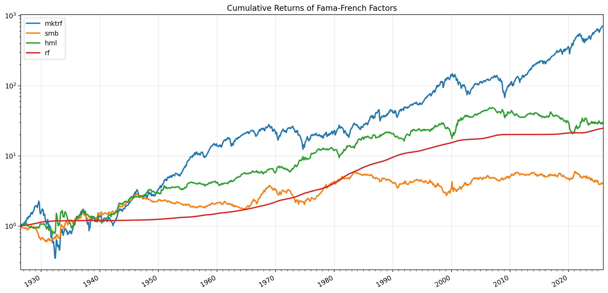
Historical returns#

ff.describe()

	mktrf	smb	hml	rf
count	1194.0	1194.0	1194.0	1194.0
mean	0.006915	0.001644	0.003473	0.0027
std	0.053074	0.031521	0.035548	0.002489
min	-0.2874	-0.1741	-0.1383	-0.0006
25%	-0.019975	-0.016275	-0.01435	0.0003
50%	0.0108	0.0006	0.0014	0.0023
75%	0.036575	0.01725	0.0176	0.0042
max	0.3881	0.3596	0.3552	0.0135

Given monthly returns, the annual return can be approximated as \(12 \times R_t\), where \(R_t\) is the return in month \(t\).

12 * ff.mean()

mktrf     0.08298
smb      0.019729
hml      0.041677
rf       0.032404
dtype: Float64

The variance of the annual return is

\[12\times\var(R_t),\]

so the volatility is

\[\sqrt{12}\times \sigma_R.\]

np.sqrt(12) * ff.std()

mktrf    0.183855
smb      0.109193
hml      0.123142
rf       0.008622
dtype: Float64

So on an annualized basis over the last 100 years, the market factor has earned a return of about 8% with a volatility of a little less than 0.2.

The Sharpe ratio is simply the average portfolio return divided by its volatility:

ff.mean() / ff.std()

mktrf    0.130289
smb      0.052157
hml      0.097702
rf       1.084899
dtype: Float64

On an annualized basis, this means we multiply by \(\sqrt{12}\).

np.sqrt(12) * ff.mean() / ff.std()

mktrf    0.451334
smb      0.180677
hml      0.338449
rf         3.7582
dtype: Float64

_images/f735fd695078a2ebe4db1f12e72a40e48db4383fff5800df9f574de9dda04514.png

The one-factor model: CAPM#

The Capital Asset Pricing Model (CAPM) says that an asset’s expected return depends on its beta, denoted \(\beta\). That is,

\[\E(R^e_i) = \beta_i \, \E(R_M^e),\]

where \(R^e_i := R_i - R_f\) is the excess return on asset \(i\) and \(R_M\) is the return on the “market portfolio.”

The CAPM is a one-factor model, where the market portfolio is the single factor — the fundamental source of risk in the economy. A factor model of returns says that the returns on an asset come from:

How much return we get from being exposed to any risk factor. In the CAPM, this is \(\E(R_M^e)\), the expected excess return from holding the market.
How much exposure to a factor we get from holding a particular asset. This is the asset’s beta, \(\beta_i = \frac{\cov(R^e_i, R^e_M)}{\var(R^e_M)}.\) It is also called the factor loading. If a stock has high factor loadings, it gives high exposure to the underlying source of risk and is therefore riskier than a stock that has a low factor loading. So high-beta stocks are riskier than low-beta stocks. This is why we say beta is a measure of an asset’s risk.

We saw above that historically the market portfolio has earned an excess return of about 8% per year. If an investor just holds the market portfolio, this is the return they earn for bearing market risk. An investor can earn a higher return by buying a stock with \(\beta_i>1\), allowing them to load up on more of the risk factor. If the investor wants to own a stocks with less risk, she buys a stock with \(\beta_i<1\) (and therefore earn a return below that of the market.

What is risk?#

The CAPM says that a high-beta stock should earn a higher return than a low beta stock. As long as arbitrage opportunities are not common in financial markets, we can only earn higher returns by taking on more risk. Therefore, the higher returns from high betas must be due to higher risk. But why is beta a measure of risk?

It is easiest to understand this if we step back and define what we mean by risk. Economically, a risky asset is one that pays off when times are “good.” This might strange, but stop and think: if you buy an insurance contract against something bad happening, are you increasing your risk or decreasing it? You should agree that insurance reduces risk. Home insurance pays you when your house burns down. It pays off in bad times. (Insurance also has a negative expected return. It has regular negative cash flows, and with a very small probability has a large positive cash flow.)

In economic models, times are “good” when people have low marginal utility. Their needs are being met. They have food to eat, and so having more food won’t increase their utility much. Times are “bad” when they have high marginal utility; their utility would increase a lot if they were able to consume more.

So a low-risk asset should be one that pays off when times are bad. It will allow you to buy more food precisely at the time that you are hungry, just like the insurance contract allows you to build a house when your house burns down. A high-risk asset pays off in good times, when you already have what you need and another dollar isn’t going to have much of an effect on your utility.

In the CAPM, the measure of whether times are good or bad is the market portfolio. This obviously ignores all kinds of important economic information about the welfare of people in an economy, but it is the measure that CAPM uses. (There are other asset pricing models that use other proxies to measure marginal utility.)

Assets with high betas must earn higher expected returns in order to incentivise investors to own these assets. People who are risk averse are willing to hold risky assets, but must be compensated for doing so.

Key fact

In the CAPM model, the measure of an asset’s risk is its beta. The bigger its beta, the more the asset loads on the single risk factor in the economy, and the higher its expected returns must be.

Estimating one-factor regressions#

We can estimate an asset’s \(\beta\) by running a time series regression,

\[R_{i,t}^e = \alpha_i + \beta_i R_{M,t}^e + \varepsilon_{i,t}.\]

The prediction of the CAPM in this context is that the \(\alpha_i\) should be zero.

# get daily Fama-French factors

ff = db.get_table('ff', 'factors_daily', 
                  columns=['date', 'mktrf', 'smb', 'hml', 'rf'], 
                  date_cols=['date']).set_index('date')

ff = ff['2015':]

# Get a list of stocks on 12/31/2015

crsp = db.raw_sql("""
                  select dlycaldt, ticker, permno, dlycap
                  from crsp.dsf_v2
                  where dlycaldt = '2015-12-31'
                    and sharetype = 'NS'
                    and securitytype = 'EQTY'
                    and securitysubtype = 'COM'
                    and usincflg = 'Y'
                    and issuertype = 'CORP'
                    and dlycap > 0
                """)

# Assign each observation to a size decile
crsp['decile'] = pd.qcut(crsp['dlycap'], 10, labels=False) + 1

crsp

	dlycaldt	ticker	permno	dlycap	decile
0	2015-12-31	EGAS	10001	78262.25	2
1	2015-12-31	AEPI	10025	393696.45	5
2	2015-12-31	JJSF	10026	2179045.59	8
3	2015-12-31	DGSE	10028	4057.68	1
4	2015-12-31	PLXS	10032	1161997.92	7
...	...	...	...	...	...
3747	2015-12-31	BSFT	93428	1028268.8	6
3748	2015-12-31	CBOE	93429	5327576.1	9
3749	2015-12-31	VLTC	93433	44975.0	2
3750	2015-12-31	SANW	93434	61920.06	2
3751	2015-12-31	TSLA	93436	31543314.25	10

3752 rows × 5 columns

# Sample 100 records from each decile
crsp_smpl = crsp.groupby('decile').apply(lambda x: x.sample(100, random_state=42)).reset_index(drop=True)

crsp_smpl

	dlycaldt	ticker	permno	dlycap	decile
0	2015-12-31	CKX	89948	19303.48	1
1	2015-12-31	MHH	92797	31820.43	1
2	2015-12-31	ONVI	87797	26505.0	1
3	2015-12-31	URRE	75672	28218.32	1
4	2015-12-31	WGA	63829	5717.32	1
...	...	...	...	...	...
995	2015-12-31	AGR	15859	9685824.0	10
996	2015-12-31	HPQ	27828	21215480.32	10
997	2015-12-31	COF	81055	38403008.1	10
998	2015-12-31	CMG	91068	14965561.8	10
999	2015-12-31	GILD	77274	143892180.0	10

1000 rows × 5 columns

# Average market cap by decile; note that cap is in thousands

crsp_smpl.groupby('decile')['dlycap'].mean()

decile
      19496.3003
      61685.4049
     123253.9379
     243560.0629
     432396.5162
     754680.4412
    1405437.5624
    2599697.0889
    5875866.3458
  49096214.9178
Name: dlycap, dtype: Float64

Next, we’ll download daily returns for every stock in our sample over the next ten years.

sql = """
      SELECT permno, ticker, dlycaldt, dlyret
      FROM crsp.dsf_v2
      WHERE permno IN %(permnos)s
      AND dlycaldt >= '2016-01-01'
      """

params = {'permnos': tuple(crsp_smpl['permno'].to_list())}

rets = db.raw_sql(sql, params=params, date_cols=['dlycaldt'])

rets = rets.pivot(index='dlycaldt', columns='permno', values='dlyret').sort_index(axis=1)

rets

permno	10001	10025	10026	10028	10032	10051	10104	10145	10158	10180	...	93132	93177	93185	93264	93266	93272	93289	93312	93339	93399
dlycaldt
2016-01-04	0.009396	-0.051329	-0.030685	-0.054546	-0.020046	-0.047416	-0.017246	-0.009655	-0.0384	0.021174	...	-0.030157	-0.0286	-0.018683	-0.044866	-0.065268	-0.029225	-0.03666	-0.027098	0.020661	0.019324
2016-01-05	-0.013298	0.016532	-0.005836	0.089744	0.0	-0.011487	-0.003077	0.00819	0.014975	0.009186	...	-0.012901	-0.001319	0.010216	0.028907	-0.012469	-0.039267	-0.049331	0.000903	0.072875	-0.009479
2016-01-06	0.014825	0.041532	0.002135	-0.073529	-0.02104	-0.005165	0.005051	-0.011314	-0.018033	0.001821	...	-0.011394	-0.012655	0.005286	-0.028095	-0.046717	-0.009537	0.156412	-0.025421	-0.049057	-0.023923
2016-01-07	0.014608	-0.038586	-0.01642	0.031746	-0.023881	-0.022713	-0.021776	-0.029441	-0.046745	-0.012461	...	-0.011186	-0.035211	-0.000229	-0.04336	-0.022517	-0.045392	-0.041667	-0.038586	-0.079365	0.0
2016-01-08	0.019634	0.004295	-0.002075	-0.015385	-0.024159	-0.041833	-0.01113	-0.008062	-0.02627	-0.014984	...	-0.019198	0.001095	0.010748	0.01983	-0.02168	0.089337	0.000669	-0.012201	0.030172	0.014706
...	...	...	...	...	...	...	...	...	...	...	...	...	...	...	...	...	...	...	...	...	...
2025-12-24	<NA>	<NA>	0.013073	0.021243	0.001366	<NA>	0.011007	0.007315	0.00033	<NA>	...	0.006447	0.005426	<NA>	0.015576	0.010345	-0.014613	-0.008479	-0.000898	<NA>	<NA>
2025-12-26	<NA>	<NA>	-0.008934	-0.03698	0.001429	<NA>	0.002532	0.002234	-0.005274	<NA>	...	0.004681	-0.014114	<NA>	-0.018405	-0.015017	-0.006408	0.010832	0.00674	<NA>	<NA>
2025-12-29	<NA>	<NA>	0.00868	0.0248	-0.018999	<NA>	-0.013183	-0.001419	-0.003645	<NA>	...	-0.009073	-0.023158	<NA>	0.003125	0.0	-0.015478	-0.00846	-0.002678	<NA>	<NA>
2025-12-30	<NA>	<NA>	-0.009378	-0.021858	-0.011303	<NA>	0.009366	-0.003704	-0.021949	<NA>	...	-0.00631	-0.001724	<NA>	0.037383	-0.003465	-0.008235	0.006826	-0.009846	<NA>	<NA>
2025-12-31	<NA>	<NA>	0.00646	0.067837	-0.017248	<NA>	-0.011663	-0.006468	-0.00408	<NA>	...	-0.011207	-0.0557	<NA>	0.012012	-0.000695	-0.001132	-0.015254	-0.012203	<NA>	<NA>

2514 rows × 1000 columns

To start, we’ll focus on the returns of just one stock — Oracle (permno 10104). We’ll merge those with the factor returns and then set up a regression.

reg = ff.merge(rets[10104], left_index=True, right_index=True)

reg['exret'] = reg[10104] - reg['rf']

# regression doesn't work NaNs
reg = reg.dropna()

# # pandas recently added a data type that doesn't play well with statsmodels so we'll convert to float
reg = reg.apply(lambda x: x.astype(float))

reg

	mktrf	smb	hml	rf	10104	exret
2016-01-04	-0.0159	-0.0087	0.0052	0.0000	-0.017246	-0.017246
2016-01-05	0.0013	-0.0018	0.0000	0.0000	-0.003077	-0.003077
2016-01-06	-0.0134	-0.0013	0.0001	0.0000	0.005051	0.005051
2016-01-07	-0.0244	-0.0029	0.0008	0.0000	-0.021776	-0.021776
2016-01-08	-0.0111	-0.0049	-0.0003	0.0000	-0.011130	-0.011130
...	...	...	...	...	...	...
2025-12-24	0.0029	0.0003	0.0001	0.0002	0.011007	0.010807
2025-12-26	-0.0006	-0.0032	0.0009	0.0002	0.002532	0.002332
2025-12-29	-0.0041	-0.0018	0.0007	0.0002	-0.013183	-0.013383
2025-12-30	-0.0020	-0.0060	0.0028	0.0002	0.009366	0.009166
2025-12-31	-0.0076	0.0007	-0.0009	0.0002	-0.011663	-0.011863

2514 rows × 6 columns

import statsmodels.api as sm

reg_model = sm.OLS(reg['exret'], sm.add_constant(reg['mktrf']))

reg_rslt = reg_model.fit()

print(reg_rslt.summary())

                            OLS Regression Results                            
==============================================================================
Dep. Variable:                  exret   R-squared:                       0.309
Model:                            OLS   Adj. R-squared:                  0.308
Method:                 Least Squares   F-statistic:                     1122.
Date:                Sun, 15 Feb 2026   Prob (F-statistic):          1.06e-203
Time:                        19:54:33   Log-Likelihood:                 6636.6
No. Observations:                2514   AIC:                        -1.327e+04
Df Residuals:                    2512   BIC:                        -1.326e+04
Df Model:                           1                                         
Covariance Type:            nonrobust                                         
==============================================================================
                 coef    std err          t      P>|t|      [0.025      0.975]
------------------------------------------------------------------------------
const          0.0003      0.000      0.945      0.345      -0.000       0.001
mktrf          0.9838      0.029     33.498      0.000       0.926       1.041
==============================================================================
Omnibus:                     2360.470   Durbin-Watson:                   2.032
Prob(Omnibus):                  0.000   Jarque-Bera (JB):           740086.464
Skew:                           3.707   Prob(JB):                         0.00
Kurtosis:                      86.727   Cond. No.                         85.2
==============================================================================

Notes:
[1] Standard Errors assume that the covariance matrix of the errors is correctly specified.

ax = reg_rslt.resid.plot(figsize=(12,6));

ax.set_xlim(reg.index.min(), reg.index.max())
ax.set_xlabel('')
ax.grid(alpha=0.3)
ax.set_title('Residuals')

plt.show()

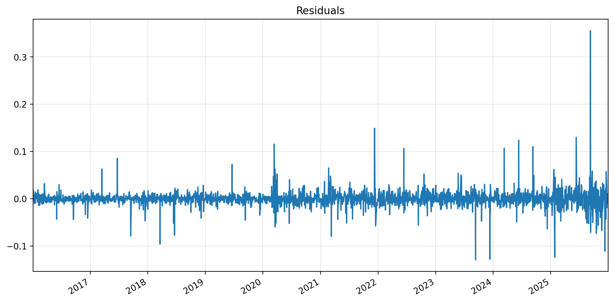
_images/9531301a3527eb32cb36377fe11e75547012beb00e89976fd82aff502bfad614.png

The volatility of the residuals give the idiosyncratic volatility of the returns.

reg_rslt.resid.std()

0.017272941420857096

Note that, by construction, the total volatility of the stock return must be greater than the idiosyncratic volatility. (This is just a different way of saying that \(RSS\leq TSS\).)

reg['exret'].std()

0.0207756215162608

The regression equation implies a decomposition of the total variance:

\[\var(R_i^e) = \beta_i^2 \var(R_M^e) + \var(\varepsilon_i).\]

Exercise

Write an expression that verifies that this equation holds for this regression.

Solution

np.isclose(reg_rslt.params['mktrf']**2 * reg['mktrf'].var() + reg_rslt.resid.var(),
           reg['exret'].var())

Fama–French 3-factor model#

The 3-factor model regression equation is:

\[R_{i,t}^e = \alpha_i + \beta^M_i R_{M,t}^e + \beta^S_i R_{SMB,t} + \beta^V_i R_{HML,t} + \varepsilon_{i,t}\]

reg_model = sm.OLS(reg['exret'],
                   sm.add_constant(reg[['mktrf', 'smb', 'hml']]))

reg_rslt = reg_model.fit()

print(reg_rslt.summary())

                            OLS Regression Results                            
==============================================================================
Dep. Variable:                  exret   R-squared:                       0.323
Model:                            OLS   Adj. R-squared:                  0.322
Method:                 Least Squares   F-statistic:                     398.9
Date:                Sun, 15 Feb 2026   Prob (F-statistic):          7.28e-212
Time:                        19:54:33   Log-Likelihood:                 6662.5
No. Observations:                2514   AIC:                        -1.332e+04
Df Residuals:                    2510   BIC:                        -1.329e+04
Df Model:                           3                                         
Covariance Type:            nonrobust                                         
==============================================================================
                 coef    std err          t      P>|t|      [0.025      0.975]
------------------------------------------------------------------------------
const          0.0003      0.000      0.800      0.424      -0.000       0.001
mktrf          1.0268      0.030     34.104      0.000       0.968       1.086
smb           -0.3549      0.052     -6.761      0.000      -0.458      -0.252
hml           -0.0879      0.037     -2.351      0.019      -0.161      -0.015
==============================================================================
Omnibus:                     2356.117   Durbin-Watson:                   2.032
Prob(Omnibus):                  0.000   Jarque-Bera (JB):           748357.886
Skew:                           3.690   Prob(JB):                         0.00
Kurtosis:                      87.201   Cond. No.                         156.
==============================================================================

Notes:
[1] Standard Errors assume that the covariance matrix of the errors is correctly specified.

reg_rslt.resid.std()

0.017096011983458715

Exercise

Notice that the idiosyncratic volatility from the three-factor model is (a little) less than it was in the one-factor model. Do you think this will always be true? Why?

def regression(permno):
    reg = ff.merge(rets[permno], left_index=True, right_index=True)
    reg['exret'] = reg[permno] - reg['rf']
    reg = reg.dropna()
    reg = reg.apply(lambda x: x.astype(float))

    reg_model = sm.OLS(reg['exret'],
                       sm.add_constant(reg[['mktrf', 'smb', 'hml']]))
    reg_rslt = reg_model.fit()
    params = reg_rslt.params
    tvals = reg_rslt.tvalues
    tvals.index = map(lambda x: 't_'+x, tvals.index)  # rename t-value index values
    rslt = pd.concat([params, tvals])
    rslt['idiovol'] = reg_rslt.resid.std()
    rslt['R2'] = reg_rslt.rsquared
    rslt['N'] = reg_rslt.nobs
    return(rslt)

regression(10104)

const         0.000273
mktrf         1.026765
smb          -0.354892
hml          -0.087928
t_const       0.800287
t_mktrf      34.103529
t_smb        -6.760801
t_hml        -2.350719
idiovol       0.017096
R2            0.322855
N          2514.000000
dtype: float64

We can now run regressions for each stock in our sample, simply by iterating over the columns of rets dataframe.

betas = {}
resids = {}
for permno in rets:
    rslt = regression(permno)
    betas[permno] = rslt

resids = pd.DataFrame(resids)

# transpose betas dataframe so coefficient estimates are columns
betas = pd.DataFrame(betas).T

betas.index.name = 'permno'

betas

/opt/anaconda3/envs/data/lib/python3.12/site-packages/statsmodels/regression/linear_model.py:1782: RuntimeWarning: divide by zero encountered in scalar divide
  return 1 - self.ssr/self.centered_tss

	N	R2	const	hml	idiovol	mktrf	smb	t_const	t_hml	t_mktrf	t_smb
permno
10001	401.0	0.004700	0.001831	0.348477	0.034141	0.077337	0.152102	1.065768	1.141784	0.306119	0.429521
10025	266.0	0.052959	0.001478	0.156676	0.036224	0.361120	1.288365	0.656756	0.397269	1.265723	2.935178
10026	2514.0	0.243397	-0.000257	0.434668	0.015573	0.628506	0.332158	-0.825597	12.757001	22.916744	6.946431
10028	2514.0	0.059242	0.002000	-0.116842	0.040246	0.581258	0.868260	2.486884	-1.326913	8.200980	7.026191
10032	2514.0	0.474473	0.000275	0.381584	0.014681	0.935942	0.898653	0.935770	11.880024	36.201666	19.936335
...	...	...	...	...	...	...	...	...	...	...	...
93272	2514.0	0.283822	0.000685	-0.240025	0.027414	1.120369	1.195174	1.250121	-4.001759	23.206363	14.198773
93289	2514.0	0.364591	-0.000096	-0.279522	0.029620	1.619436	1.130870	-0.163033	-4.313268	31.046068	12.434518
93312	2514.0	0.478956	-0.000040	0.090056	0.012845	1.021770	0.189439	-0.154002	3.204478	45.169867	4.803289
93339	2190.0	0.051517	-0.000048	0.062933	0.049997	0.758708	0.854044	-0.044591	0.551746	8.131942	5.227847
93399	768.0	0.011111	-0.001056	0.677137	0.067454	-0.597287	-0.298509	-0.432363	1.539241	-2.051509	-0.616744

1000 rows × 11 columns

betas['mktrf'].plot.hist(bins=25, edgecolor='k');

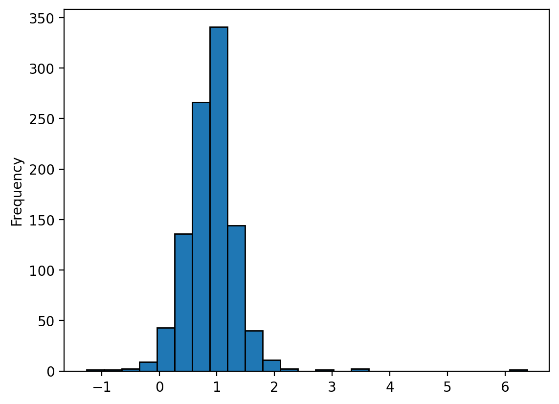
_images/16be8460ad999a6f0557acbb6c39549d72c8da4ce213a51ccaea273127d06b50.png

betas['mktrf'].mean()

0.8982117048905841

# Add stock names to the betas dataframe

names = db.get_table('crsp', 'stocknames', columns=['permno', 'comnam', 'nameenddt'], date_cols=['nameenddt'])

# Keep only the last name for each permno
names = names.groupby('permno').last()

betas = betas.merge(names, left_index=True, right_index=True)

betas[betas['mktrf']<0].sort_values('mktrf')

	N	R2	const	hml	idiovol	mktrf	smb	t_const	t_hml	t_mktrf	t_smb	comnam	nameenddt
permno
92805	83.0	0.025865	-0.002946	1.504742	0.099863	-1.264681	1.803016	-0.262254	0.842205	-1.181817	0.894746	TIANYIN PHARMACEUTICAL CO INC	2016-04-29
12509	452.0	0.002087	0.006419	0.658607	0.137706	-0.735246	-0.168119	0.983660	0.552994	-0.742823	-0.121706	WOLVERINE BANCORP INC	2017-10-16
93399	768.0	0.011111	-0.001056	0.677137	0.067454	-0.597287	-0.298509	-0.432363	1.539241	-2.051509	-0.616744	NATIONAL AMERICAN UNIV HLDGS INC	2019-01-18
15292	366.0	0.033693	0.001854	0.283895	0.016705	-0.440383	0.150763	2.104024	1.772076	-3.266097	0.814962	CARDCONNECT CORP	2017-07-05
13970	814.0	0.003625	0.001215	-0.261854	0.052162	-0.270108	0.421342	0.662382	-0.789101	-1.219093	1.145360	TRUETT HURST INC	2019-03-27
88257	495.0	0.014157	0.001129	0.465077	0.024545	-0.256056	0.261237	1.015032	2.276387	-1.478651	1.108905	PEOPLES FINANCIAL CORP MS	2017-12-15
59192	10.0	0.228028	-0.002826	-0.920269	0.007992	-0.158150	0.345276	-0.475726	-0.773162	-0.517802	0.299794	CHUBB CORP	2016-01-14
12922	191.0	0.070417	0.001682	0.289971	0.034447	-0.152218	1.998889	0.667511	0.629909	-0.521535	3.666602	SKULLCANDY INC	2016-10-03
90954	390.0	0.000587	0.002236	0.064411	0.047161	-0.136648	0.189104	0.929387	0.151369	-0.391066	0.381752	SAJAN INC	2017-07-19
14880	292.0	0.008853	0.004246	-0.810888	0.056288	-0.129838	0.426573	1.273035	-1.365786	-0.296054	0.651811	WAFERGEN BIO SYSTEMS INC	2017-02-28
15011	884.0	0.002241	0.000342	0.042635	0.016072	-0.073369	-0.041232	0.629508	0.434761	-1.107577	-0.378958	MELROSE BANCORP INC	2019-07-08
83762	2464.0	0.022696	-0.001237	-1.018439	0.069745	-0.068131	0.794118	-0.878637	-6.642836	-0.542151	3.685498	AIM IMMUNOTECH INC	2024-12-31
15905	621.0	0.000233	0.001361	0.165555	0.084723	-0.052705	0.200668	0.397848	0.251666	-0.115932	0.288514	NAKED BRAND GROUP INC	2018-06-19

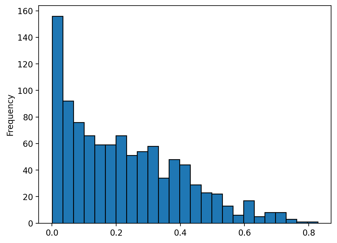
betas['R2'].describe()

count    1000.000000
mean            -inf
std              NaN
min             -inf
25%         0.066643
50%         0.195681
75%         0.341969
max         0.828717
Name: R2, dtype: float64

betas[betas['R2'] < 0.0]

	N	R2	const	hml	idiovol	mktrf	smb	t_const	t_hml	t_mktrf	t_smb	comnam	nameenddt
permno
47088	1.0	-inf	NaN	-0.71047	NaN	2.172398	1.18867	NaN	-0.0	0.0	0.0	KANSAS CITY LIFE INS CO	2015-12-31

betas = betas.drop(47088)

betas['R2'].plot.hist(bins=25, edgecolor='k');

_images/818557d297523024fe32467dd36ab5672c8906f9d0de30f4f20a6e9858b8ef01.png

betas[betas['R2']>0.7]

	N	R2	const	hml	idiovol	mktrf	smb	t_const	t_hml	t_mktrf	t_smb	comnam	nameenddt
permno
10932	2514.0	0.717934	-0.000057	1.420335	0.013391	1.361483	0.782681	-0.212183	48.479595	57.734119	19.036142	WEBSTER FINANCIAL CORP	2024-12-31
35044	2514.0	0.746665	0.000121	1.349310	0.011505	1.298547	0.523922	0.528387	53.604703	64.091542	14.831443	REGIONS FINANCIAL CORP NEW	2024-12-31
47896	2514.0	0.728335	0.000210	0.892704	0.009058	1.139786	-0.169259	1.162418	45.044981	71.451985	-6.085798	JPMORGAN CHASE & CO	2024-12-31
66157	2514.0	0.707452	-0.000225	1.093414	0.010319	1.122059	0.147498	-1.089499	48.430625	61.745204	4.655304	U S BANCORP DEL	2024-12-31
71563	2514.0	0.719005	-0.000195	1.198307	0.011222	1.238374	0.308653	-0.869878	48.803316	62.659223	8.957321	TRUIST FINANCIAL CORP	2024-12-31
76624	10.0	0.755154	0.001325	0.535250	0.003929	0.518561	-0.654305	0.453867	0.914690	3.453483	-1.155578	P M C SIERRA INC	2016-01-14
76684	2514.0	0.745275	0.000123	1.487470	0.012616	1.307638	0.896711	0.486731	53.890514	58.857750	23.149540	HANCOCK WHITNEY CORP	2024-12-31
80808	30.0	0.828717	0.000751	1.076955	0.008316	1.060967	0.770422	0.446386	4.733552	9.252303	2.454555	METRO BANCORP INC	2016-02-12
81564	1133.0	0.768737	0.000275	1.666323	0.013799	1.372409	0.964430	0.669330	31.113339	40.372397	13.562480	IBERIABANK CORP	2020-07-01
86004	1802.0	0.716823	-0.000103	1.156500	0.011686	1.108619	0.737802	-0.375276	40.969616	48.727848	17.090251	UMPQUA HOLDINGS CORP	2023-02-28
86382	2514.0	0.720587	-0.000077	1.153640	0.010462	0.928959	0.927366	-0.370439	50.398813	50.419518	28.868681	FIRST BUSEY CORP	2024-12-31
88197	2514.0	0.709473	-0.000018	1.257466	0.011364	1.044199	0.767379	-0.077457	50.573076	52.174549	21.991694	FULTON FINANCIAL CORP PA	2024-12-31

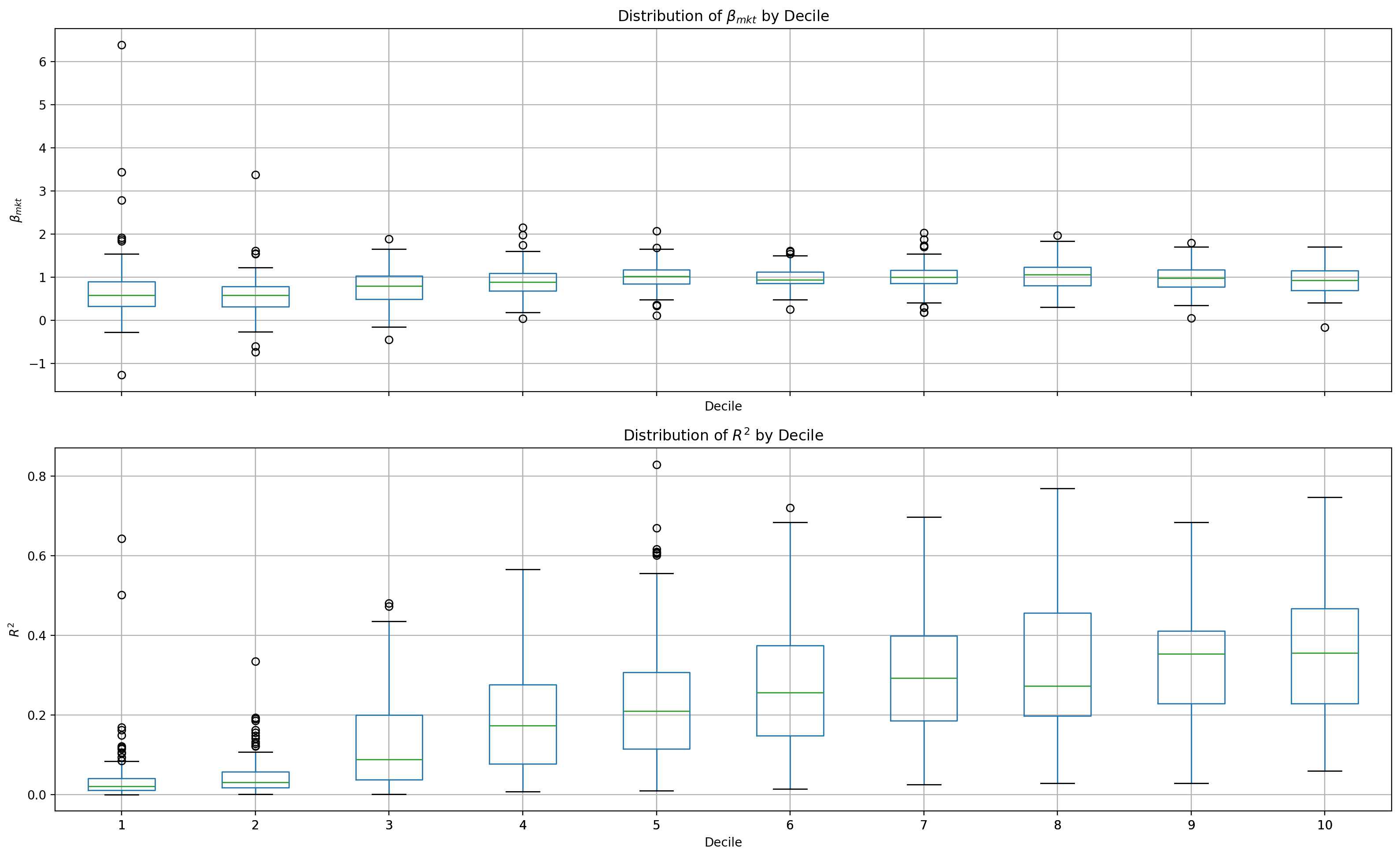
Next, we’ll generate a box-and-whiskers plot, which summarizes the distribution of estimated market betas within each size decile. For each decile, the box shows the median and interquartile range, while the whiskers show outliers of betas, highlighting how market exposure varies across firm sizes.

# add back the decile information
betas = betas.merge(crsp_smpl[['permno', 'decile']], left_index=True, right_on='permno')

fig, axes = plt.subplots(2, 1, figsize=(16, 10), sharex=True)

betas.boxplot(column='mktrf', by='decile', ax=axes[0])
betas.boxplot(column='R2', by='decile', ax=axes[1])

for i, col in enumerate(['mktrf', 'R2']):
    axes[i].set_xlabel('Decile')
    label = r'$\beta_{mkt}$' if col == 'mktrf' else r'$R^2$'
    axes[i].set_ylabel(label)
    axes[i].set_title(f'Distribution of {label} by Decile')

fig.suptitle('')
fig.tight_layout()
plt.show()

_images/ce208dfc41f08fca6cc601f86db6f7a432467b11bf474eae1e9a397f1a337e57.png

Are alphas zero?#

betas['const'].describe()

count    999.000000
mean       0.000240
std        0.012683
min       -0.106850
25%       -0.000215
50%        0.000128
75%        0.000518
max        0.381501
Name: const, dtype: float64

To determine whether the \(\alpha_i\) are statistically different from zero, we divide the average \(\alpha\) by the standard error of the mean, \(\sigma/\sqrt{n}\), to calculate a \(t\)-statistic.

import scipy.stats as scs

print("SEM:\t{:.4f}".format(scs.sem(betas['const'])))

print("t-stat:\t{:.2f}".format(betas['const'].mean() / scs.sem(betas['const'])))

SEM:	0.0004
t-stat:	0.60

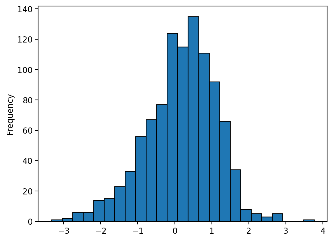
betas['t_const'].plot.hist(bins=25, edgecolor='k');

_images/18830f7122a0e5fe7f88ac53367f4441e341290a2c887cc72d1a9fc061b124b5.png