Covariance

Consider the variance of the sum of two random variables,

\[\begin{align*} \var(X+Y) &= \E[(X+Y)^2] - [\E(X+Y)]^2 \\ &= \E[X^2 + 2XY + Y^2] - \left[\E(X)^2 + 2\E(X)\E(Y) + \E(Y)^2\right] \\ &= \E(X^2) + 2\E(XY) + \E(Y^2) - \E(X)^2 - 2\E(X)\E(Y) - \E(Y)^2 \\ &= \var(X) + \var(Y) + 2[\E(XY) - \E(X)\E(Y)] \end{align*}\]

Clearly, the variance equals the sum of the two variances, plus an additional term involving the product of the two random variables. This term is the covariance, which measures the tendency of two random variables to move together. It’s defined as

\[\begin{align*} \cov(X,Y) &:= \E[(X-\E(X))(Y-\E(Y))] \\ &= \E(XY) - \E(X)\E(Y). \end{align*}\]

Note

In general, \(\E(XY) \neq \E(X)\E(Y),\) since

\[\int f(x y)\,dx\,dy \neq \left(\int f(x) \,dx\right) \left(\int f(y) \,dy\right),\]

except in special cases.

Exercise

Show that:

1. \(\cov(X,Y) = \cov(Y,X)\)

2. \(\cov(X,X) = \var(X)\)

3. \(\cov(aX,bY) = ab\cov(X,Y)\)

4. \(\cov(a+X,b+Y) = \cov(X,Y)\)

Note that facts #2 and #3 imply that \(\var(bX) = b^2\var(X)\), as we saw earlier.

The variance–covariance matrix

It will often be useful to think about variance and covariance simultaenously for multiple variables, which is easiest to do in a matrix context. Suppose that \(X\) and \(Y\) are random variables, and let \(Z = \begin{pmatrix}X\\Y\end{pmatrix}\). The variance of \(Z\) is

\[\begin{align*} \var(Z) &= \E(Z^2) - \E(Z)^2 \\ &= \E(ZZ') - \E(Z)\E(Z)'. \end{align*}\]

Therefore,

\[\begin{align*} \var\left[\begin{pmatrix} X\\ Y \end{pmatrix}\right] &= \E\left[\begin{pmatrix} X\\ Y \end{pmatrix} \begin{pmatrix} X & Y \end{pmatrix}\right] - \E\left[\begin{pmatrix} X\\ Y \end{pmatrix}\right] \E\left[\begin{pmatrix} X & Y \end{pmatrix}\right]\\ &= \E\begin{pmatrix} X^2 & XY \\ XY & Y^2 \end{pmatrix} - \begin{pmatrix} \E(X)^2 & \E(XY) \\ \E(XY) & \E(Y)^2 \end{pmatrix} \\ &= \begin{pmatrix} \E(X^2) - \E(X)^2 & \E(XY) - \E(X)\E(Y) \\ \E(XY) - \E(X)\E(Y) & \E(Y^2)-\E(Y)^2 \end{pmatrix} \\ &= \begin{pmatrix} \var(X) & \cov(X,Y) \\ \cov(X,Y) & \var(Y) \end{pmatrix}. \end{align*}\]

This is the variance–covariance matrix, often denoted \(\boldsymbol{\Sigma}\). It contains information about all the variances and covariances for the cross terms. Since we have two random variables, the matrix is \(2\times 2\).

The variance–covariance matrix can be defined for an arbitrary number of variables. For example, suppose we have \(n\) random variables, \(X_1, X_2, \ldots, X_n.\) The variance–covariance matrix is

\[\begin{align*} \boldsymbol{\Sigma} = \var \, \left[\begin{pmatrix} X_1\\ X_2 \\ \vdots \\ X_n \end{pmatrix} \right] &= \begin{pmatrix} \var(X_1) & \cov(X_1,X_2) & \cdots & \cov(X_1,X_n) \\ \cov(X_2,X_1) & \var(X_2) & \cdots & \cov(X_2,X_n) \\ \vdots & \vdots & \ddots & \vdots \\ \cov(X_n,X_1) & \cov(X_n,X_2) & \cdots & \var(X_n) \end{pmatrix} \\ &= \begin{pmatrix} \sigma^2_1 & \sigma_{12} & \cdots & \sigma_{1n} \\ \sigma_{21} & \sigma^2_2 & \cdots & \sigma_{2n} \\ \vdots & \vdots & \ddots & \vdots \\ \sigma_{n1} & \sigma_{n2} & \cdots & \sigma^2_n \end{pmatrix}, \end{align*}\]

where \(\sigma_{ij} := \cov(X_i,X_j).\) The matrix is clearly square, with \(n\) rows and \(n\) columns, as well as symmetric about the diagonal, since \(\sigma_{ij} = \sigma_{ji}\).

Correlation

Correlation is a scaled measure of covariance calculated as

\[\begin{equation*} \rho _{X,Y}=\operatorname {corr} (X,Y)= {\cov(X,Y) \over \sigma_{X}\sigma _{Y}} = {\E[(X-\mu_X)(Y-\mu_Y)] \over \sigma_X \sigma_Y}. \end{equation*}\]

The triangle inequality, which says that the sum of the lengths of any two sides of a triangle must be greater than the length of the third, is a consequence of the Cauchy–Schwartz inequality.

An important result in math, called the Cauchy–Schwarz inequality, says that

\[\left[\cov(X,Y)\right]^2 \leq \var(X)\var(Y),\]

implying that

\[\frac{|\cov(X,Y)|}{\sigma_X\sigma_Y} \leq 1 \quad\Longrightarrow \quad |\rho_{X,Y}| \leq 1.\]

Correlation must therefore lie in the interval \([-1,1]\).

We use the following terms to describe how \(X\) and \(Y\) are related, given their correlation.

\(\rho_{X,Y}\)	Meaning
\(\rho = -1\)	Perfectly negatively correlated
\(\rho < 0\)	Negatively correlated
\(\rho = 0\)	Uncorrelated
\(\rho > 0\)	Positively correlated
\(\rho = 1\)	Perfectly positively correlated

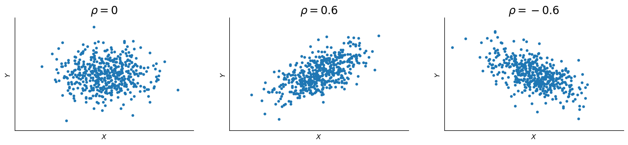
The figure below shows the correlation of three simulated datasets. In each panel, we take 500 random draws for two variables \(X\) and \(Y\) that are each normally distributed but have a correlation of \(\rho\). Each \((x_i, y_i)\) pair is plotted. In the left panel, the data are uncorrelated and there is no obvious pattern between the the values of \(x_i\) and \(y_i\). Both values tend to be near zero, but when one value is high or low, it doesn’t tell us anything about whether the other value is high or low.

In the second panel, with correlation of 0.6, there is a clear positive relation: when \(x_i\) is high, \(y_i\) also tends to be high; and when \(x_i\)is low, \(y_i\) tends also to be low. In the third panel, the pattern is flipped, so high values of \(x_i\) are generally paired with low values of \(y_i\), and vice versa.

Show code cell source

Hide code cell source

# The following correlation plots are adapted from code at
# https://commons.wikimedia.org/wiki/File:Correlation_examples2.svg

import matplotlib.pyplot as plt
import numpy as np
from numpy import pi as π
from numpy import cos, sin, sqrt

rng = np.random.default_rng()

def plot(ax, xy, xlim=(-4,4), ylim=(-4,4)):
    ax.scatter(xy[:,0], xy[:,1], marker='.')
    ax.set_xlim(xlim)
    ax.set_ylim(ylim)
    return ax

fig, axes = plt.subplots(1,3,figsize=(16,3))

μ = np.array([0,0])

# Top row: vary correlation
N = 500
for ax,ρ in zip(axes, [0, 0.6, -0.6]):
    Σ = np.array([[1, ρ], [ρ, 1]])
    xy = rng.multivariate_normal(μ, Σ, N)
    ax = plot(ax, xy)
    ax.set_title(r'$\rho={}$'.format(ρ), fontsize=16)
    
# Formatting
for ax in axes.ravel():
    ax.xaxis.set_ticks([])
    ax.yaxis.set_ticks([])
    ax.set_xlabel('$X$')
    ax.set_ylabel('$Y$')    
    for s in ['right', 'top']:
        ax.spines[s].set_visible(False)    

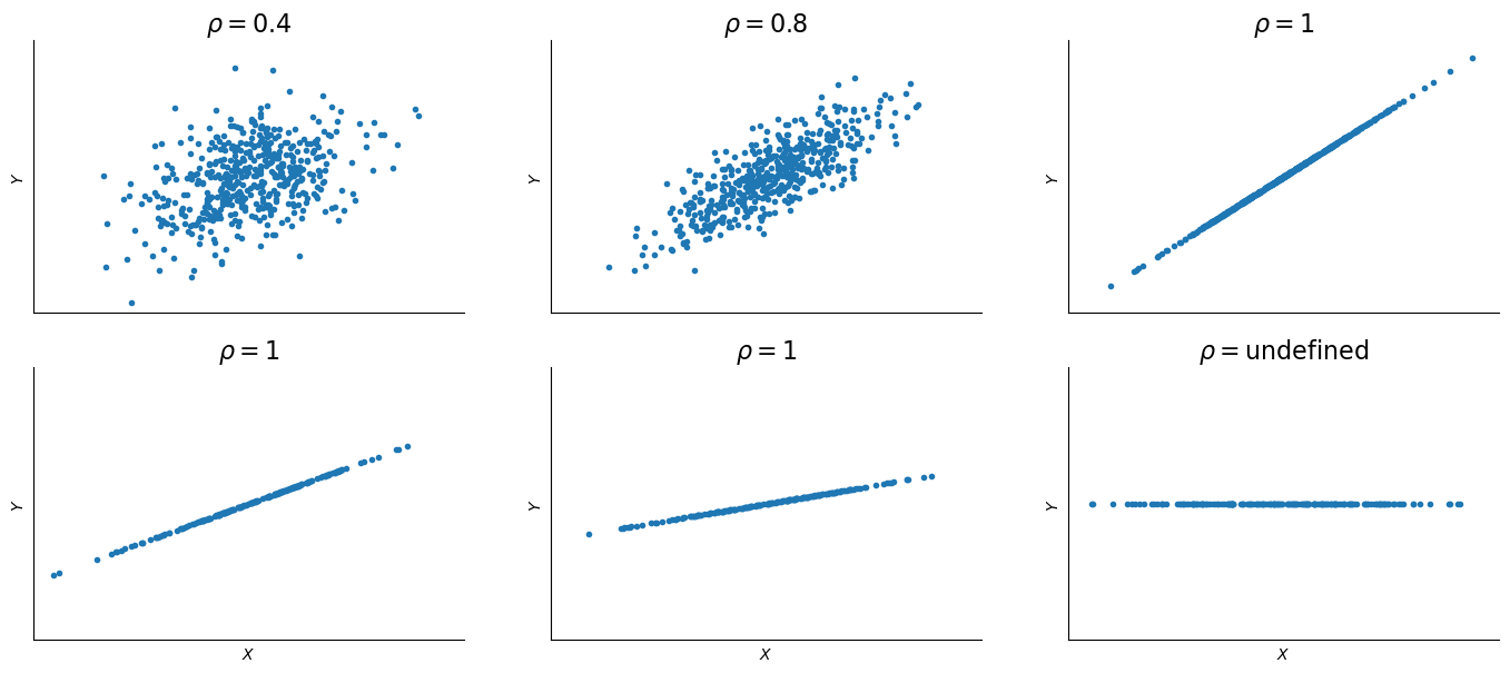
As we increase correlation, the connection between the two random variables becomes tighter, as can be seen in the plots below. When variables are perfectly correlated, they move exactly together, so the data line up on a straight line. The slope of the line need not be 45°. In the lower right panel, \(Y\) does not vary, so \(\sigma_Y=0\) and correlation cannot be calculated (although covariance is zero).

Show code cell source

Hide code cell source

def rotate(θ, X):
    '''Rotate matrix X by θ'''
    return X @ np.array([[cos(θ), -sin(θ)],
                         [sin(θ),  cos(θ)]])

fig, axes = plt.subplots(2,3,figsize=(17,7))

μ = np.array([0,0])

N = 500
for ax,ρ in zip(axes[0], [0.4, 0.8, 1]):
    Σ = np.array([[1, ρ], [ρ, 1]])
    xy = rng.multivariate_normal(μ, Σ, N)
    ax = plot(ax, xy)
    ax.set_title(r'$\rho={}$'.format(ρ), fontsize=16)

N = 200
Σ = np.array([[1, 1], [1, 1]])
for ax,θ,lbl in zip(axes[1],
                    [π/12, π/6,     π/4],
                    [   1,   1, 'undefined']):
    xy = rng.multivariate_normal(μ, Σ, N)
    xy = rotate(θ, xy)
    ax = plot(ax, xy)
    ax.set_title((r'$\rho={}$' if isinstance(lbl, int) else r'$\rho=${}').format(lbl), fontsize=16)

# Formatting
for i,ax in enumerate(axes.ravel()):
    ax.xaxis.set_ticks([])
    ax.yaxis.set_ticks([])
    ax.set_ylabel('$Y$')
    if i>=3:
        ax.set_xlabel('$X$')
    for s in ['right', 'top']:
        ax.spines[s].set_visible(False)

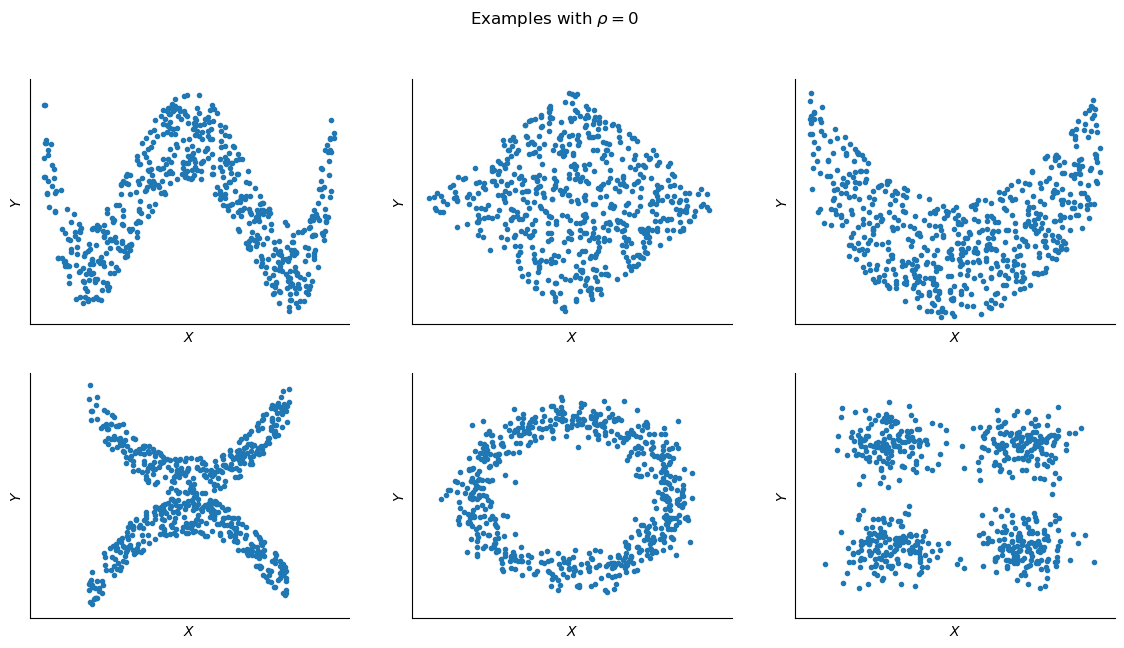
If the variables are independent, the correlation coefficient is 0, but the converse is not true because the correlation coefficient detects only linear dependencies between two variables. This is depicted in the figure below, which provides six examples of data where there is clearly some relation between \(X\) and \(Y\) despite all having a correlation of zero. In all of these cases, the dependence between the variables is nonlinear, and correlation cannot detect such patterns.

Show code cell source

Hide code cell source

fig, axes = plt.subplots(2,3,figsize=(14,7))
plt.suptitle(r'Examples with $\rho=0$')

N = 600
μ = np.array([0,0])

axes = axes.ravel()

# W shape
ax = axes[0]
x = rng.uniform(-1, 1, N)
y = 4 * (x**2 - 1/2)**2 + rng.uniform(-1, 1, N)/3
xy = np.c_[(x,y)]
ax = plot(ax, xy, (-1,1), (-1/3, 1+1/3))

# diamond
ax = axes[1]
y = rng.uniform(-1, 1, N)
xy = rotate(-π/4, np.c_[(x,y)])
lims = (-sqrt(2), sqrt(2))
ax = plot(ax, xy, lims, lims)

# U shape
ax = axes[2]
y = 2*x**2 + rng.uniform(-1, 1, N)
ax = plot(ax, np.c_[(x,y)], (-1,1), (-1,3))

# X shape
ax = axes[3]
y = (x**2 + rng.uniform(0, 0.5, N)) * np.random.choice([-1, 1], N)
ax = plot(ax, np.c_[(x,y)], (-1.5, 1.5), (-1.5, 1.5))

# O shape
ax = axes[4]
y = cos(x*π) + np.random.normal(0, 1/8, N)
x = sin(x*π) + np.random.normal(0, 1/8, N)
ax = plot(ax, np.c_[(x,y)], (-1.5, 1.5), (-1.5, 1.5))

# clusters
ax = axes[5]
xy1 = rng.multivariate_normal(np.array([ 3,  3]), np.eye(2), int(N/4))
xy2 = rng.multivariate_normal(np.array([-3,  3]), np.eye(2), int(N/4))
xy3 = rng.multivariate_normal(np.array([-3, -3]), np.eye(2), int(N/4))
xy4 = rng.multivariate_normal(np.array([ 3, -3]), np.eye(2), int(N/4))
xy = np.r_[(xy1, xy2, xy3, xy4)]
ax = plot(ax, xy, (-7,7), (-7,7))
                              
# Formatting
for ax in axes:
    ax.xaxis.set_ticks([])
    ax.yaxis.set_ticks([])
    ax.set_xlabel('$X$')
    ax.set_ylabel('$Y$')
    xlim = ax.get_xlim()
    ax.set_xlim(xlim[0]-0.1, xlim[1]+0.1)
    ylim = ax.get_ylim()
    ax.set_ylim(ylim[0]-0.1, ylim[1]+0.1)
    for s in ['right', 'top']:
        ax.spines[s].set_visible(False)

The fact that two random variables can be uncorrelated even if they are not independent is sometimes misunderstood, even by very smart people who should know better. For an interesting recent example, see this tweet and additional discussion on this blog.

Formally, the relation between independence and correlation is

\[\begin{equation*} \begin{aligned} X,Y{\text{ independent}}\quad &\Rightarrow \quad \rho _{X,Y}=0, \\ \rho _{X,Y}=0\quad &\nRightarrow \quad X,Y{\text{ independent}}. \end{aligned} \end{equation*}\]

Note, however, that if either \(X\) or \(Y\) are constant (``non-stochastic’’) then their correlation will be undefined even though they are independent.

Key fact

Correlation can range from \(-1\) to \(1\). It is zero whenever \(X\) and \(Y\) are independent random variables, although it can also be zero even if they are not independent.