
Volatility modeling#
import numpy as np
import pandas as pd
import matplotlib.pyplot as plt
import wrds

db = wrds.Connection()
Loading library list...
Done
import statsmodels.api as sm

from statsmodels.tsa.arima.model import ARIMA
from statsmodels.tsa.stattools import acf, pacf

# This code will supress certain unnecessary warnings from the statsmodels package
import warnings
from statsmodels.tools.sm_exceptions import ValueWarning
warnings.filterwarnings('ignore', module='statsmodels', category=FutureWarning)
warnings.filterwarnings('ignore', module='statsmodels', category=ValueWarning)
We’ll be using the arch package, so be sure to have that installed.
from arch import arch_model
from arch.univariate import ARX, GARCH, EGARCH, ConstantMean, StudentsT, SkewStudent
sql = """
    SELECT dlycaldt, dlyret
    FROM crsp.dsf_v2
    WHERE ticker = 'SPY' AND dlycaldt >= '1992-01-01'
"""

spy = db.raw_sql(sql, date_cols=['dlycaldt']).set_index('dlycaldt').dropna().sort_index()

spy = spy.squeeze()
spy.name = 'ret'
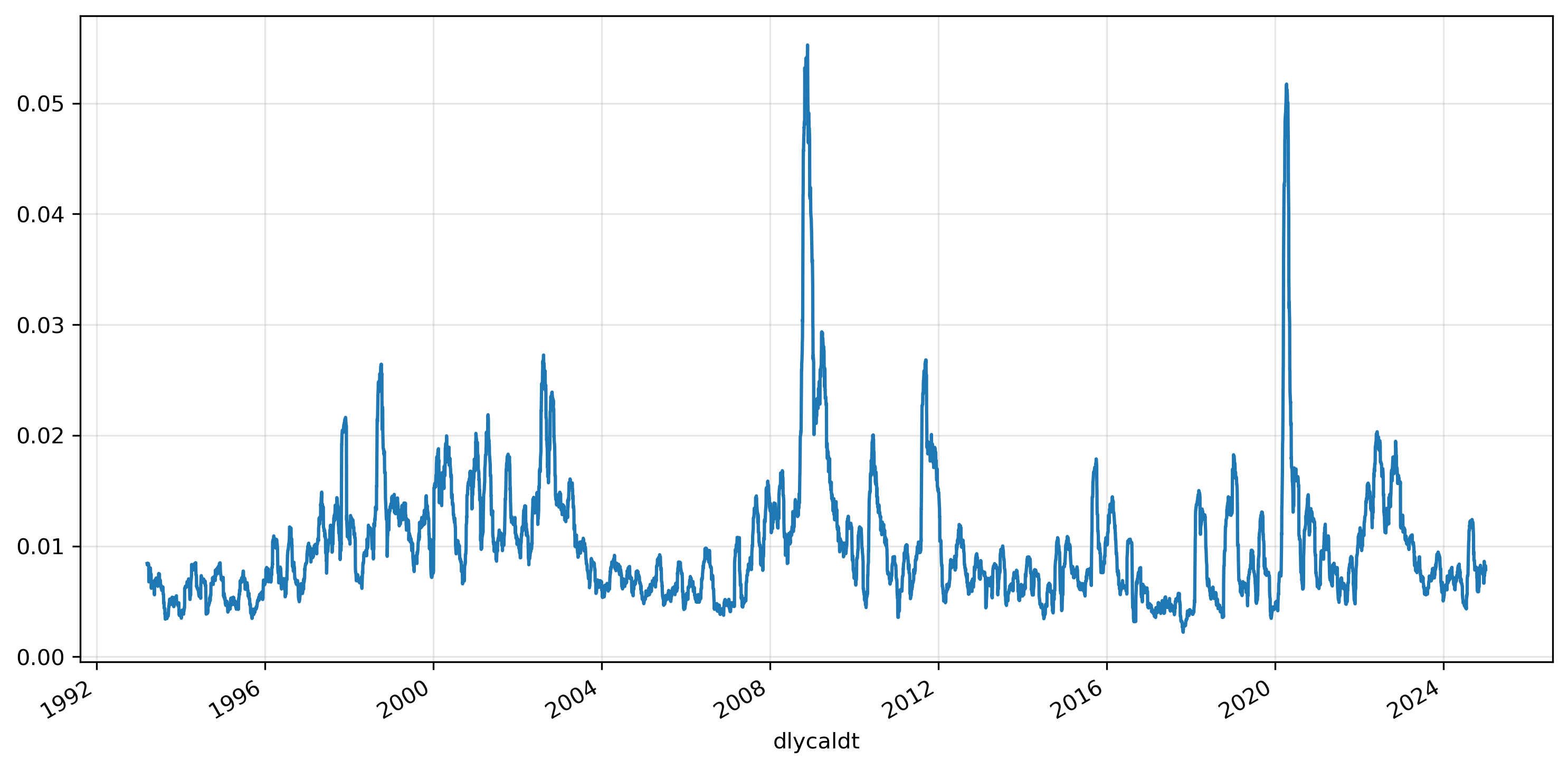
spy.rolling(30).std().plot(grid=True);
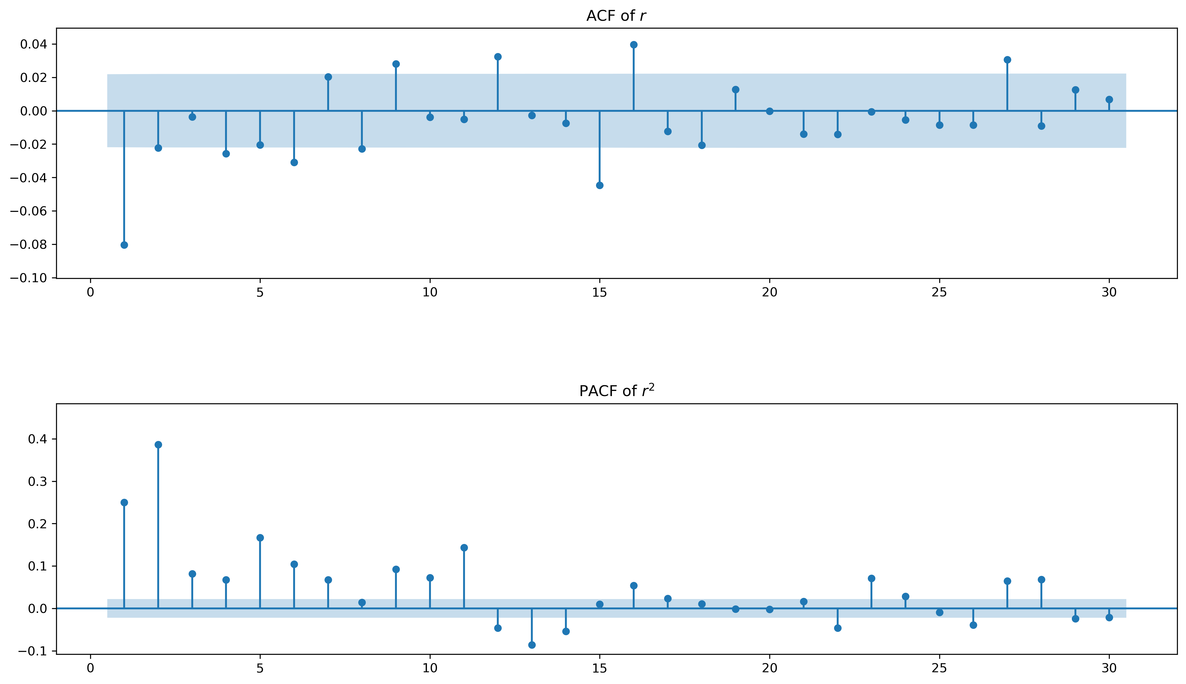
fig, (ax1,ax2) = plt.subplots(2,1,figsize=(16,9))

fig = sm.graphics.tsa.plot_acf(spy, lags=30, zero=False, auto_ylims=True, ax=ax1)
ax1.set_title('ACF of $r$')

fig = sm.graphics.tsa.plot_pacf(spy**2, lags=30, ax=ax2, zero=False, auto_ylims=True)
ax2.set_title('PACF of $r^2$')

plt.subplots_adjust(hspace=0.5)
plt.show()
GARCH#
If we specify an ARMA model for \(\sigma^2\), the model is called a generalized autoregressive conditional heteroskedasticity (GARCH) model.
Notice that as \(\sigma_t\) changes, the volatility of \(\varepsilon_t\) changes. Obviously, if \(\sigma_t=1\) then \(\varepsilon_t=e_t\) has a variance of 1. But suppose that \(\sigma_t=1.5\). Now
so the volatility of \(\varepsilon_t\) is 1.5. In other words, the volatility of the noise term is controlled entirely by \(\sigma_t\), which we allow to vary over time.
More generally, a GARCH(\(p,q\)) model specifies a variance of
# scaling helps with log-likelihood maximization
spy = spy*100
mod1 = ConstantMean(spy)
mod1.volatility = GARCH(p=1,q=1)
res1 = mod1.fit(disp='on')
print(res1.summary())
Iteration:      1,   Func. Count:      6,   Neg. LLF: 20062887524.700806
Iteration:      2,   Func. Count:     15,   Neg. LLF: 4466900010.967097
Iteration:      3,   Func. Count:     22,   Neg. LLF: 15260.542033681926
Iteration:      4,   Func. Count:     29,   Neg. LLF: 412871363.43178666
Iteration:      5,   Func. Count:     36,   Neg. LLF: 10990.878452086183
Iteration:      6,   Func. Count:     42,   Neg. LLF: 10888.236448941509
Iteration:      7,   Func. Count:     48,   Neg. LLF: 10996.484425467956
Iteration:      8,   Func. Count:     54,   Neg. LLF: 10864.646830478745
Iteration:      9,   Func. Count:     59,   Neg. LLF: 10959.529518585998
Iteration:     10,   Func. Count:     65,   Neg. LLF: 10864.334592763795
Iteration:     11,   Func. Count:     70,   Neg. LLF: 10864.327018863847
Iteration:     12,   Func. Count:     75,   Neg. LLF: 10864.326967600262
Iteration:     13,   Func. Count:     80,   Neg. LLF: 10864.326964939455
Iteration:     14,   Func. Count:     84,   Neg. LLF: 10864.32696493941
                     Constant Mean - GARCH Model Results
==============================================================================
Dep. Variable:                    ret   R-squared:                       0.000
Mean Model:             Constant Mean   Adj. R-squared:                  0.000
Vol Model:                      GARCH   Log-Likelihood:               -10864.3
Distribution:                  Normal   AIC:                           21736.7
Method:            Maximum Likelihood   BIC:                           21764.6
                                        No. Observations:                 8037
Date:                Wed, Apr 23 2025   Df Residuals:                     8036
Time:                        09:26:54   Df Model:                            1
                                 Mean Model
============================================================================
                 coef    std err          t      P>|t|      95.0% Conf. Int.
----------------------------------------------------------------------------
mu             0.0753  8.903e-03      8.456  2.770e-17 [5.783e-02,9.273e-02]
                              Volatility Model
============================================================================
                 coef    std err          t      P>|t|      95.0% Conf. Int.
----------------------------------------------------------------------------
omega          0.0206  4.078e-03      5.058  4.229e-07 [1.264e-02,2.862e-02]
alpha[1]       0.1126  1.159e-02      9.711  2.719e-22   [8.984e-02,  0.135]
beta[1]        0.8720  1.227e-02     71.079      0.000     [  0.848,  0.896]
============================================================================

Covariance estimator: robust
The estimated model is
Notice that \(\alpha+\beta \approx 1\). This is commonly observed with financial data, and the related IGARCH model requires \(\alpha+\beta=1\) as a constraint in the estimation.
res1.params
mu          0.075280
omega       0.020628
alpha[1]    0.112557
beta[1]     0.871952
Name: params, dtype: float64
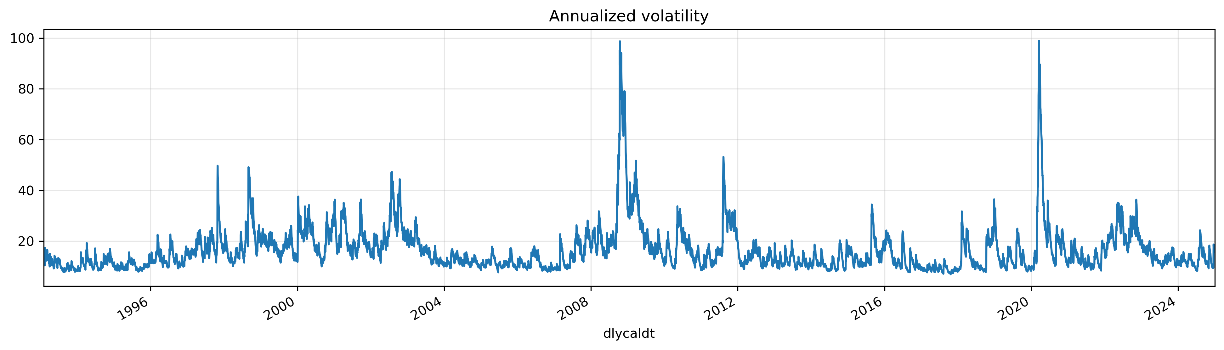
The conditional volatility is the estimate of the time series of \(\sigma^2\).
res1.conditional_volatility
dlycaldt
1993-02-01    0.774564
1993-02-02    0.767641
1993-02-03    0.732493
1993-02-04    0.772639
1993-02-05    0.744587
                ...
2024-12-24    1.061264
2024-12-26    1.059975
2024-12-27    1.000418
2024-12-30    1.018096
2024-12-31    1.044503
Name: cond_vol, Length: 8037, dtype: float64
(res1.conditional_volatility * np.sqrt(252)).plot(figsize=(16, 4), grid=True)

plt.xlim(spy.index[0], spy.index[-1])
plt.title('Annualized volatility')
plt.show()
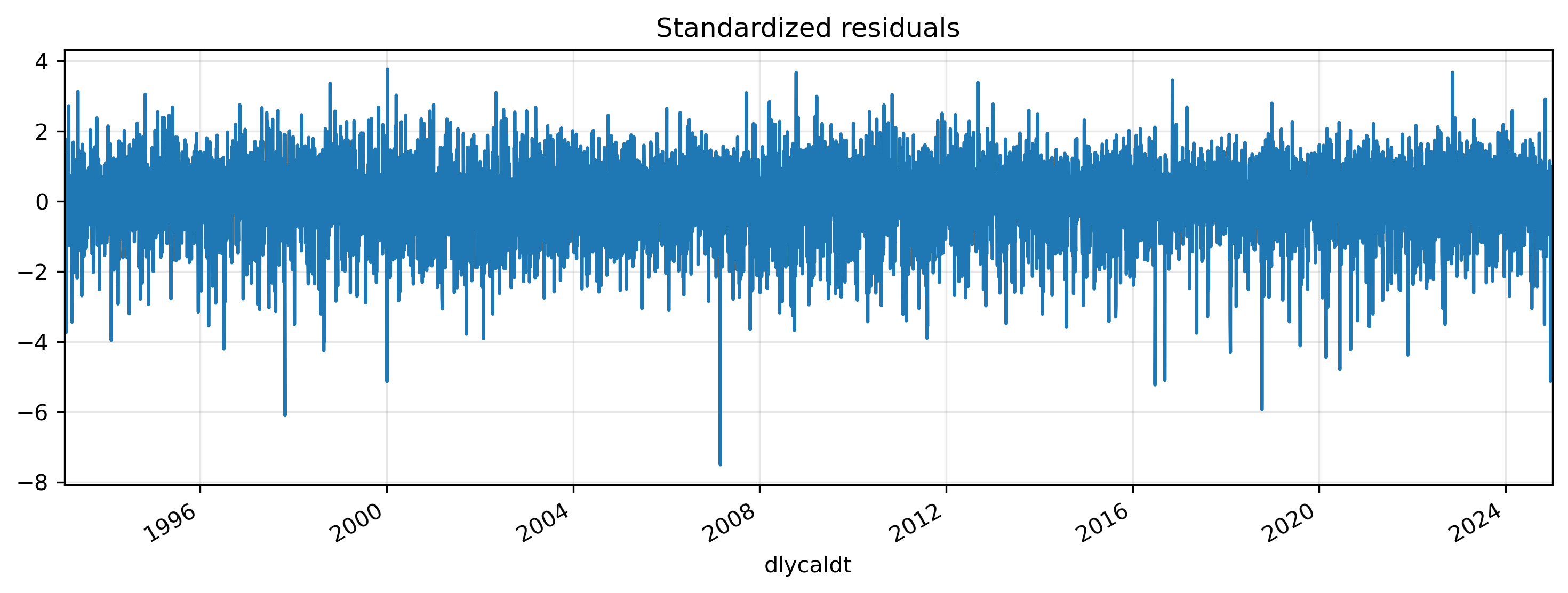
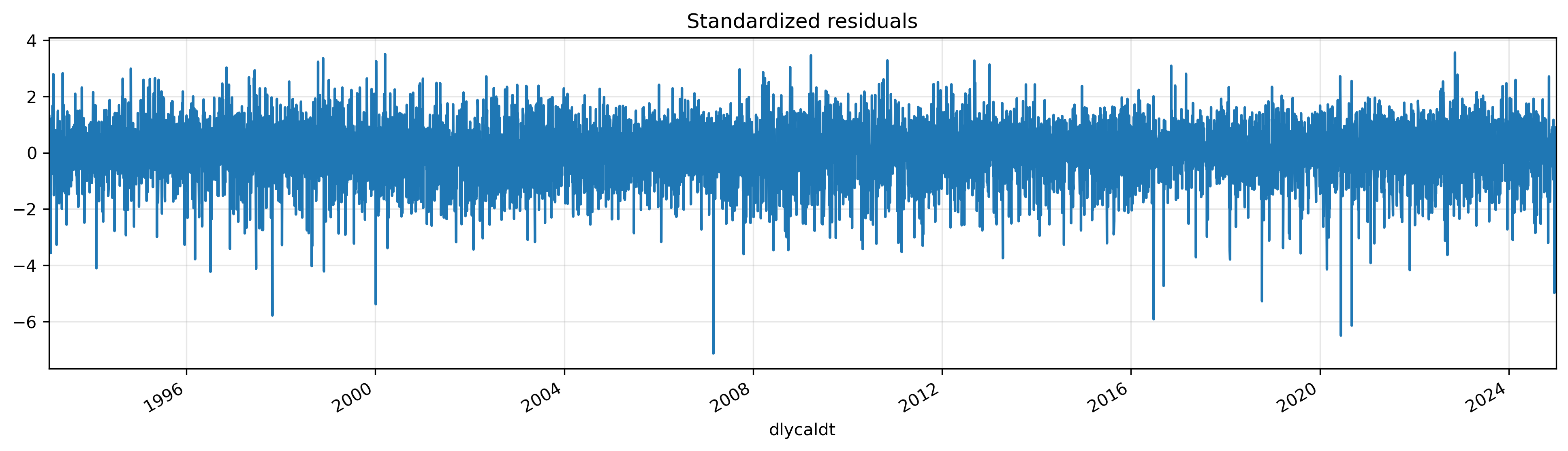
std_resid = res1.resid / res1.conditional_volatility
std_resid.plot(figsize=(16,4), grid=True)
plt.xlim(spy.index[0], spy.index[-1])
plt.title('Standardized residuals')
plt.show();
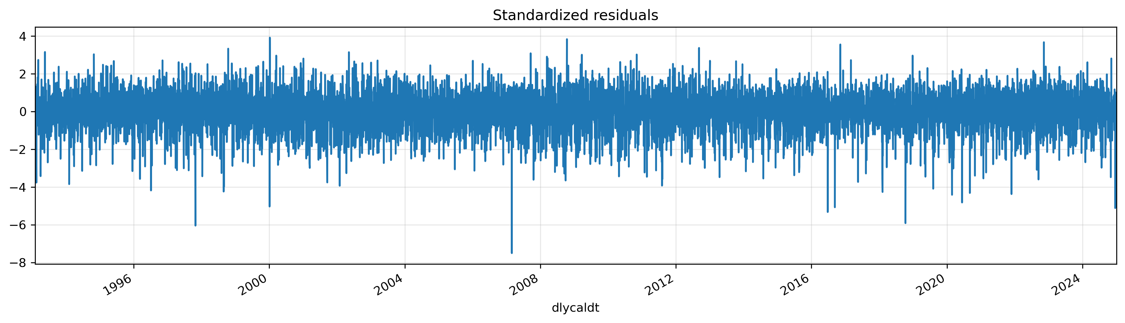
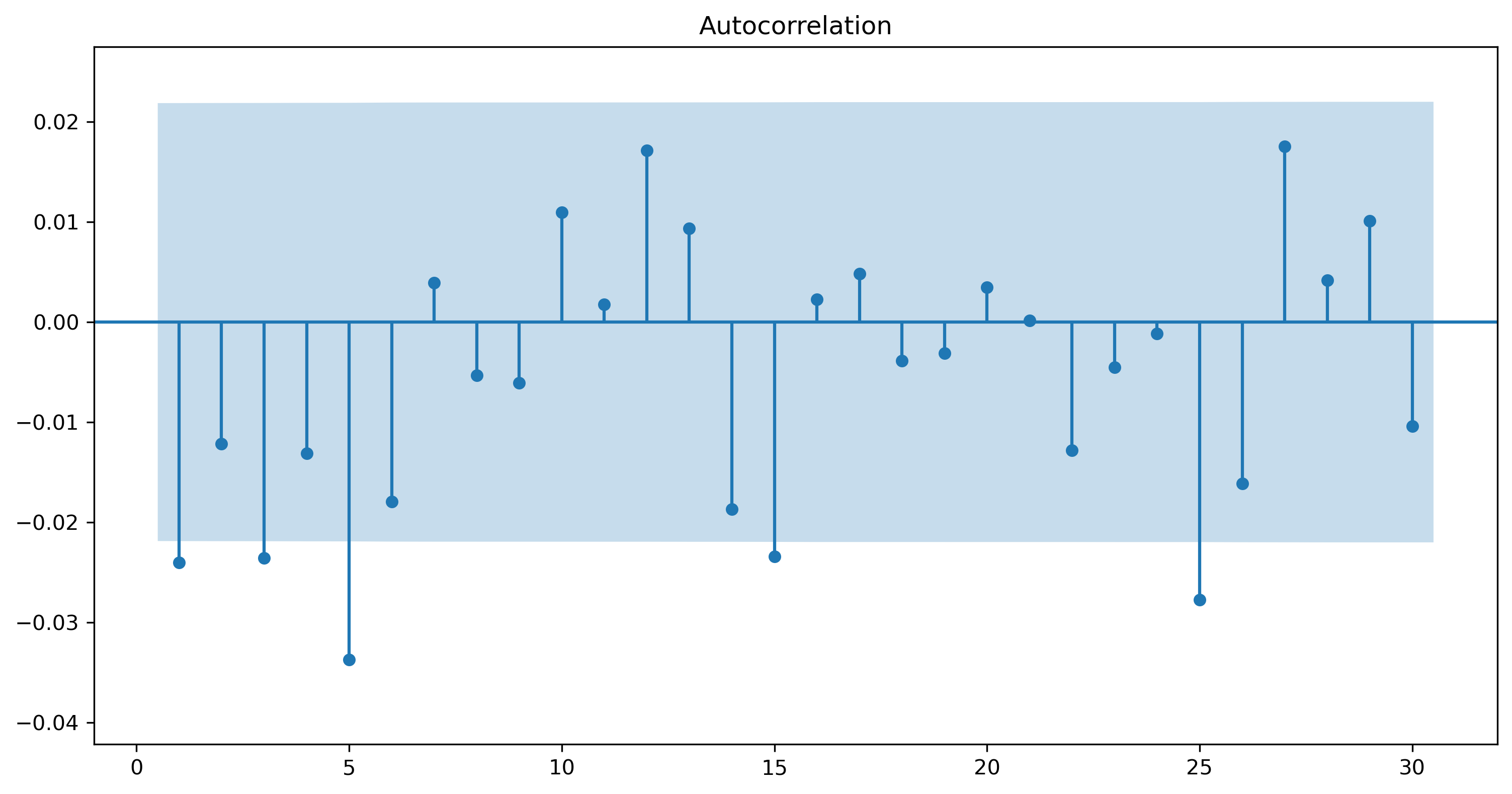
fig = sm.graphics.tsa.plot_acf(std_resid.values, lags=30, zero=False, auto_ylims=True)
We don’t have to assume a constant mean for the return process. Instead, we can combine an AR process in the return with GARCH volatility. For example, we can fit an AR(3) model to the data. We’ll start with just an AR(3), and then add in the GARCH process for the volatility.
ar3 = ARIMA(spy, order=(3,0,0)).fit()

print(ar3.summary())
                               SARIMAX Results
==============================================================================
Dep. Variable:                    ret   No. Observations:                 8037
Model:                 ARIMA(3, 0, 0)   Log Likelihood              -12642.957
Date:                Wed, 23 Apr 2025   AIC                          25295.913
Time:                        09:31:31   BIC                          25330.872
Sample:                             0   HQIC                         25307.876
                               - 8037
Covariance Type:                  opg
==============================================================================
                 coef    std err          z      P>|z|      [0.025      0.975]
------------------------------------------------------------------------------
const          0.0461      0.012      3.735      0.000       0.022       0.070
ar.L1         -0.0829      0.006    -13.956      0.000      -0.095      -0.071
ar.L2         -0.0296      0.005     -6.379      0.000      -0.039      -0.021
ar.L3         -0.0080      0.006     -1.387      0.165      -0.019       0.003
sigma2         1.3611      0.009    150.470      0.000       1.343       1.379
===================================================================================
Ljung-Box (L1) (Q):                   0.00   Jarque-Bera (JB):             38747.82
Prob(Q):                              0.98   Prob(JB):                         0.00
Heteroskedasticity (H):               0.87   Skew:                            -0.20
Prob(H) (two-sided):                  0.00   Kurtosis:                        13.75
===================================================================================

Warnings:
[1] Covariance matrix calculated using the outer product of gradients (complex-step).
mod2 = ARX(spy, lags=3)
mod2.volatility = GARCH(p=1,q=1)
res2 = mod2.fit(disp='off')
print(res2.summary())
                           AR - GARCH Model Results
==============================================================================
Dep. Variable:                    ret   R-squared:                       0.004
Mean Model:                        AR   Adj. R-squared:                  0.003
Vol Model:                      GARCH   Log-Likelihood:               -10852.4
Distribution:                  Normal   AIC:                           21718.8
Method:            Maximum Likelihood   BIC:                           21767.7
                                        No. Observations:                 8034
Date:                Wed, Apr 23 2025   Df Residuals:                     8030
Time:                        09:31:46   Df Model:                            4
                                  Mean Model
==============================================================================
                 coef    std err          t      P>|t|        95.0% Conf. Int.
------------------------------------------------------------------------------
Const          0.0818  9.455e-03      8.650  5.134e-18     [6.326e-02,  0.100]
ret[1]        -0.0371  1.192e-02     -3.110  1.870e-03 [-6.044e-02,-1.371e-02]
ret[2]        -0.0173  1.294e-02     -1.337      0.181  [-4.266e-02,8.062e-03]
ret[3]        -0.0303  1.235e-02     -2.451  1.425e-02 [-5.448e-02,-6.065e-03]
                              Volatility Model
============================================================================
                 coef    std err          t      P>|t|      95.0% Conf. Int.
----------------------------------------------------------------------------
omega          0.0205  4.096e-03      5.012  5.393e-07 [1.250e-02,2.856e-02]
alpha[1]       0.1118  1.172e-02      9.539  1.443e-21   [8.881e-02,  0.135]
beta[1]        0.8727  1.243e-02     70.204      0.000     [  0.848,  0.897]
============================================================================

Covariance estimator: robust
In a model with \(k\) lags of the time series, the conditional volatility will be missing for \(k\) periods.
res2.conditional_volatility
dlycaldt
1993-02-01         NaN
1993-02-02         NaN
1993-02-03         NaN
1993-02-04    0.796735
1993-02-05    0.769729
                ...
2024-12-24    1.054962
2024-12-26    1.058383
2024-12-27    0.999064
2024-12-30    1.012957
2024-12-31    1.041451
Name: cond_vol, Length: 8037, dtype: float64
We can “prune” the model by dropping insignificant parameters.
mod2 = ARX(spy, lags=[1,3])
mod2.volatility = GARCH(p=1,q=1)
res2 = mod2.fit(disp='off')
print(res2.summary())
                           AR - GARCH Model Results
==============================================================================
Dep. Variable:                    ret   R-squared:                       0.003
Mean Model:                        AR   Adj. R-squared:                  0.003
Vol Model:                      GARCH   Log-Likelihood:               -10853.4
Distribution:                  Normal   AIC:                           21718.9
Method:            Maximum Likelihood   BIC:                           21760.8
                                        No. Observations:                 8034
Date:                Wed, Apr 23 2025   Df Residuals:                     8031
Time:                        09:32:21   Df Model:                            3
                                  Mean Model
==============================================================================
                 coef    std err          t      P>|t|        95.0% Conf. Int.
------------------------------------------------------------------------------
Const          0.0804  9.277e-03      8.668  4.408e-18   [6.223e-02,9.860e-02]
ret[1]        -0.0365  1.190e-02     -3.068  2.154e-03 [-5.984e-02,-1.319e-02]
ret[3]        -0.0299  1.232e-02     -2.427  1.521e-02 [-5.406e-02,-5.759e-03]
                              Volatility Model
============================================================================
                 coef    std err          t      P>|t|      95.0% Conf. Int.
----------------------------------------------------------------------------
omega          0.0206  4.087e-03      5.039  4.670e-07 [1.259e-02,2.861e-02]
alpha[1]       0.1121  1.166e-02      9.613  7.060e-22   [8.926e-02,  0.135]
beta[1]        0.8723  1.237e-02     70.494      0.000     [  0.848,  0.897]
============================================================================

Covariance estimator: robust
std_resid2 = res2.resid / res2.conditional_volatility

ax = std_resid2.plot(figsize=(12,4), grid=True)
plt.xlim(spy.index[0], spy.index[-1])
plt.title('Standardized residuals')
plt.show()
<>:5: SyntaxWarning: invalid escape sequence '\h'
<>:10: SyntaxWarning: invalid escape sequence '\h'
<>:5: SyntaxWarning: invalid escape sequence '\h'
<>:10: SyntaxWarning: invalid escape sequence '\h'
/var/folders/8b/3b5yf0214zvg3prfcqs6wx3c0000gq/T/ipykernel_34885/12402403.py:5: SyntaxWarning: invalid escape sequence '\h'
  ax1.set_title('ACF of $\hat{e}$')
/var/folders/8b/3b5yf0214zvg3prfcqs6wx3c0000gq/T/ipykernel_34885/12402403.py:10: SyntaxWarning: invalid escape sequence '\h'
  ax2.set_title('ACF of $\hat{e}^2$')
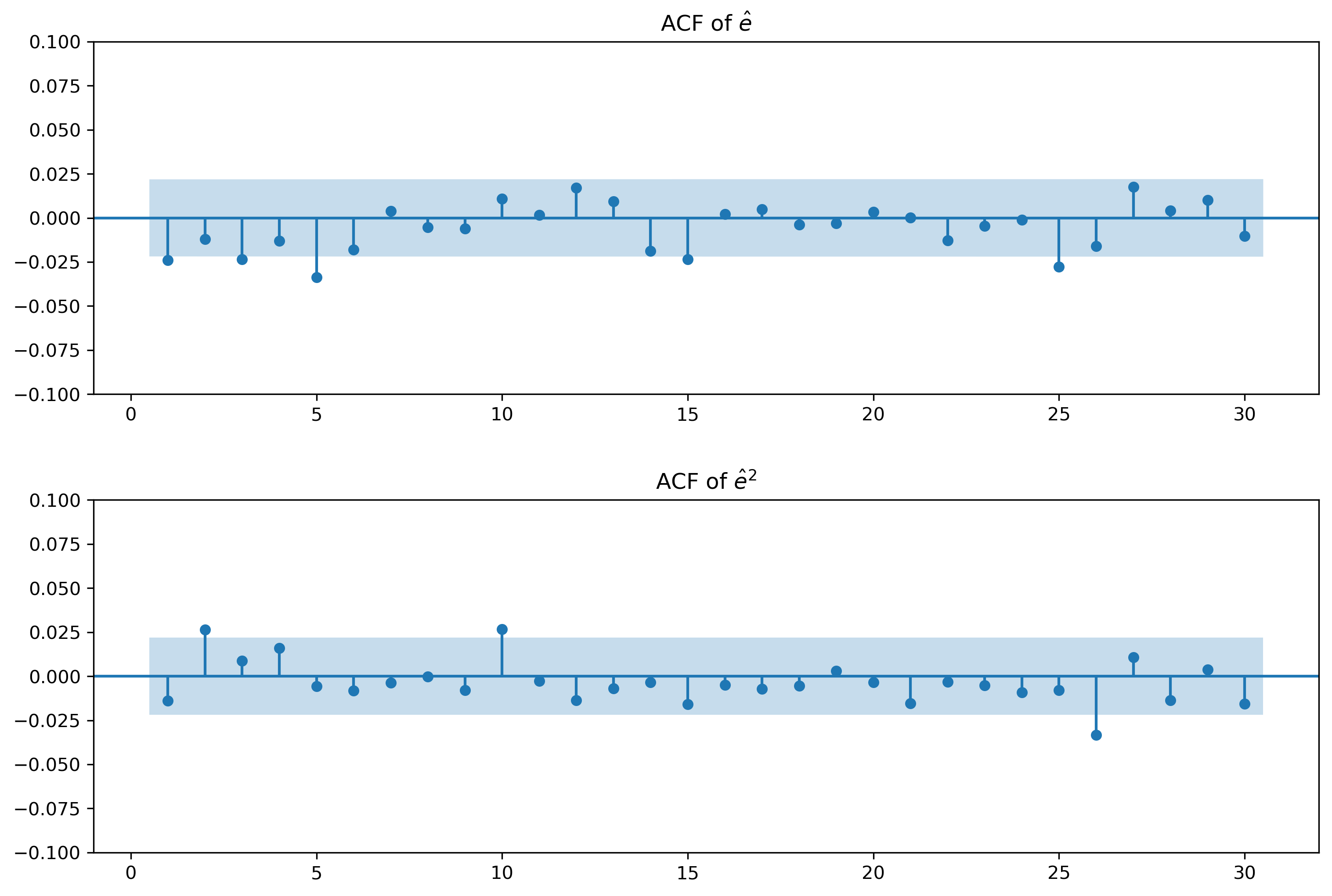
acfn, qstats, pvals = acf(std_resid, qstat=True, nlags=15)

pvals
array([0.0312882 , 0.05431309, 0.01626493, 0.01993702, 0.00087765,
       0.00067057, 0.00137535, 0.00251076, 0.00420409, 0.00528902,
       0.00894994, 0.00672621, 0.00869598, 0.00566077, 0.00219161])
acfn, qstats, pvals = acf(std_resid**2, qstat=True, nlags=15)

pvals
array([0.2082051 , 0.026455  , 0.05056582, 0.0409472 , 0.06895238,
       0.10024628, 0.15057953, 0.21706441, 0.25550552, 0.07400785,
       0.10384168, 0.1058008 , 0.13347933, 0.17488681, 0.13722661])
EGARCH#
The EGARCH(\(p,q\)) model specifies the log-volatility process as follows:
where
Modeling the log of volatility ensures that volatility is always positive, so no additional constraints are required. And the weighted error structure allows for an asymmetric effect of a return innovation on the volatility:
That is, when an innovation \(e_{t-k}\) is positive, log-variance increases by \(\alpha_k(\theta+\lambda)\), but when the innovation is negative the log-variance decreases by \(\alpha_k(\theta-\lambda)\). This asymmetry allows for a “leverage effect” as we’ll soon see. (In either case, we also reduce the log-variance by \(\lambda E(|e_t|)\), which we’ll soon see is simply a number we can calculate.)
The arch package parameterizes the model as EGARCH(\(p,o,q\)) with
Comparing (18) and (19), we see that:
implementing the typical EGARCH(\(p,q\)) model implies that \(p=o\);
\(\gamma_k\) maps to \(\theta\alpha_k\) in equation (1); and
\(\alpha_k\) (in equation 2) maps to \(\lambda\alpha_k\) in equation (1).
The \(\gamma_k\) parameter is called the leverage parameter. If \(\gamma_k=0\) then there is no asymmetry in the volaility — positive and negative values of \(e_t\) have the same effect on \(\sigma_t^2\). If, however, \(\gamma<0\), then negative shocks will lead to larger increases in volatility than positive shocks.
Error distributions#
Three distributions are often used for the innovation \(e_t\):
the Normal distribution;
the Student’s T distribution; or
the Generalized Error Distribution.
Each distributional assumption leads to a different value of \(E(|e_{t}|)\). With a Normal distribution we have
from scipy.stats import norm, t
from numpy import pi as π
# calculate E(|e|) for e~N(0,1)

norm().expect(lambda x: np.abs(x))
np.float64(0.7978845608028655)
np.sqrt(2/π)
np.float64(0.7978845608028654)
With a Student’s T distribution,
where \(\Gamma(z)\) is the gamma function.
def exp_abs_e(ν):
    """Calculate E(|e_t|) for a Student's T distribution"""
    from scipy.special import gamma as Γ
    return (2 * np.sqrt(ν-2) * Γ((ν+1)/2)) / ((ν-1) * Γ(ν/2) * np.sqrt(π))
df = 5

exp_abs_e(df)
np.float64(0.7351051938957227)
# standardized T-distribution
s = 1/np.sqrt(df/(df-2))
t_std = t(df=df, scale=s)

t_std.expect(lambda x: np.abs(x))
np.float64(0.7351051938957227)
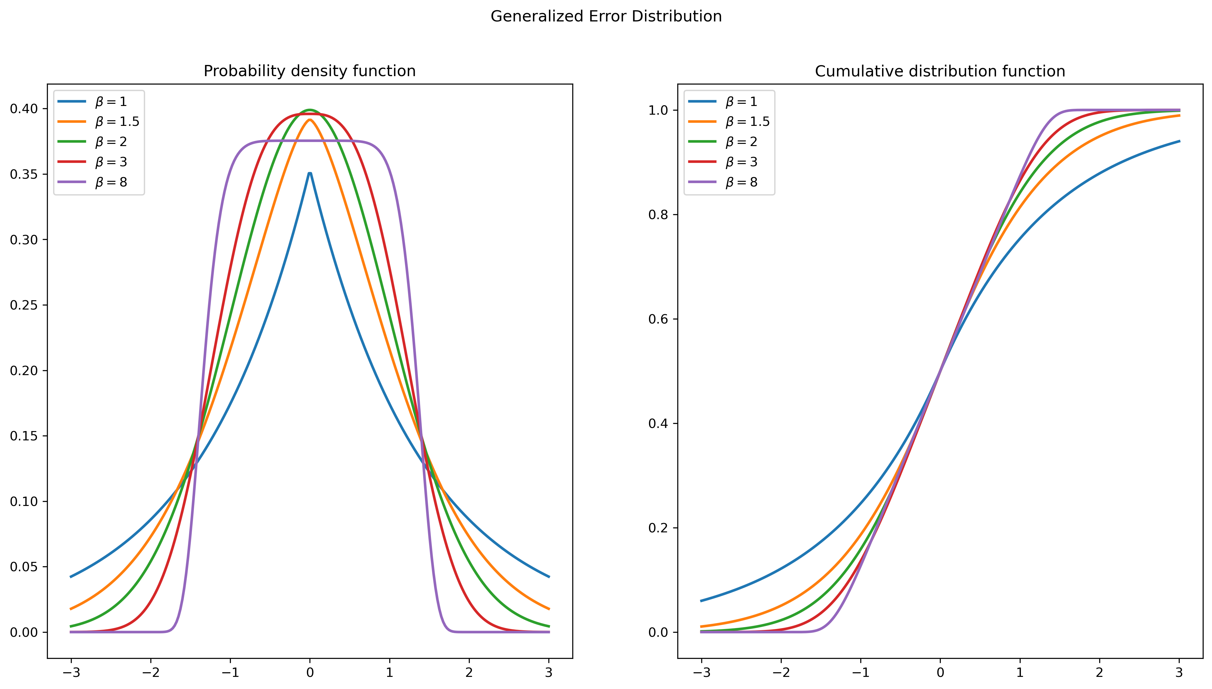
The Generalized Error Distribution is an alternative distribution that nests the Normal distribution, as well as several other continuous distributions.
Estimation#
mod3 = ARX(spy, lags=1)
mod3.volatility = EGARCH(1,1,1)
res3 = mod3.fit()
print(res3.summary())
Iteration:      1,   Func. Count:      8,   Neg. LLF: 658936358519798.0
Iteration:      2,   Func. Count:     20,   Neg. LLF: 659173899730214.5
Iteration:      3,   Func. Count:     31,   Neg. LLF: 13060330235107.09
Iteration:      4,   Func. Count:     42,   Neg. LLF: 567638731477.8679
Iteration:      5,   Func. Count:     53,   Neg. LLF: 5037293988613.256
Iteration:      6,   Func. Count:     64,   Neg. LLF: 37499.435287587694
Iteration:      7,   Func. Count:     74,   Neg. LLF: 10832.126223824762
Iteration:      8,   Func. Count:     82,   Neg. LLF: 10695.267458503542
Iteration:      9,   Func. Count:     89,   Neg. LLF: 10695.264292207961
Iteration:     10,   Func. Count:     96,   Neg. LLF: 10695.264193180004
Iteration:     11,   Func. Count:    103,   Neg. LLF: 10695.264191980066
Iteration:     12,   Func. Count:    109,   Neg. LLF: 10695.26419197779
Optimization terminated successfully    (Exit mode 0)
            Current function value: 10695.264191980066
            Iterations: 12
            Function evaluations: 109
            Gradient evaluations: 12
                          AR - EGARCH Model Results
==============================================================================
Dep. Variable:                    ret   R-squared:                       0.004
Mean Model:                        AR   Adj. R-squared:                  0.004
Vol Model:                     EGARCH   Log-Likelihood:               -10695.3
Distribution:                  Normal   AIC:                           21402.5
Method:            Maximum Likelihood   BIC:                           21444.5
                                        No. Observations:                 8036
Date:                Wed, Apr 23 2025   Df Residuals:                     8034
Time:                        09:35:59   Df Model:                            2
                                  Mean Model
==============================================================================
                 coef    std err          t      P>|t|        95.0% Conf. Int.
------------------------------------------------------------------------------
Const          0.0445  8.833e-03      5.037  4.729e-07   [2.718e-02,6.180e-02]
ret[1]        -0.0293  1.244e-02     -2.354  1.858e-02 [-5.365e-02,-4.898e-03]
                               Volatility Model
=============================================================================
                 coef    std err          t      P>|t|       95.0% Conf. Int.
-----------------------------------------------------------------------------
omega      1.1732e-03  2.615e-03      0.449      0.654 [-3.953e-03,6.299e-03]
alpha[1]       0.1633  1.539e-02     10.606  2.784e-26      [  0.133,  0.193]
gamma[1]      -0.1349  1.358e-02     -9.936  2.891e-23      [ -0.162, -0.108]
beta[1]        0.9718  4.199e-03    231.447      0.000      [  0.964,  0.980]
=============================================================================

Covariance estimator: robust
mod4 = ARX(spy, lags=1)
mod4.volatility = EGARCH(2,2,2)
res4 = mod4.fit(disp='off')
print(res4.summary())
                          AR - EGARCH Model Results
==============================================================================
Dep. Variable:                    ret   R-squared:                       0.005
Mean Model:                        AR   Adj. R-squared:                  0.005
Vol Model:                     EGARCH   Log-Likelihood:               -10672.8
Distribution:                  Normal   AIC:                           21363.6
Method:            Maximum Likelihood   BIC:                           21426.6
                                        No. Observations:                 8036
Date:                Wed, Apr 23 2025   Df Residuals:                     8034
Time:                        09:36:12   Df Model:                            2
                                  Mean Model
==============================================================================
                 coef    std err          t      P>|t|        95.0% Conf. Int.
------------------------------------------------------------------------------
Const          0.0440  6.668e-03      6.599  4.150e-11   [3.093e-02,5.707e-02]
ret[1]        -0.0408  7.131e-03     -5.728  1.015e-08 [-5.482e-02,-2.687e-02]
                               Volatility Model
=============================================================================
                 coef    std err          t      P>|t|       95.0% Conf. Int.
-----------------------------------------------------------------------------
omega      1.5742e-03  2.624e-03      0.600      0.549 [-3.568e-03,6.717e-03]
alpha[1]       0.0431  4.314e-02      0.998      0.318   [-4.149e-02,  0.128]
alpha[2]       0.1319  7.768e-02      1.698  8.960e-02   [-2.039e-02,  0.284]
gamma[1]      -0.2048  1.806e-02    -11.341  8.235e-30      [ -0.240, -0.169]
gamma[2]       0.0760  5.247e-02      1.448      0.147   [-2.684e-02,  0.179]
beta[1]        0.9700      0.307      3.159  1.584e-03      [  0.368,  1.572]
beta[2]        0.0000      0.298      0.000      1.000      [ -0.584,  0.584]
=============================================================================

Covariance estimator: robust
mod5 = ARX(spy, lags=1)
mod5.volatility = EGARCH(1,1,1)
mod5.distribution = StudentsT()
res5 = mod5.fit(disp='off')
print(res5.summary())
                             AR - EGARCH Model Results
====================================================================================
Dep. Variable:                          ret   R-squared:                       0.004
Mean Model:                              AR   Adj. R-squared:                  0.004
Vol Model:                           EGARCH   Log-Likelihood:               -10521.6
Distribution:      Standardized Student's t   AIC:                           21057.2
Method:                  Maximum Likelihood   BIC:                           21106.2
                                              No. Observations:                 8036
Date:                      Wed, Apr 23 2025   Df Residuals:                     8034
Time:                              09:36:14   Df Model:                            2
                                  Mean Model
==============================================================================
                 coef    std err          t      P>|t|        95.0% Conf. Int.
------------------------------------------------------------------------------
Const          0.0646  8.224e-03      7.856  3.976e-15   [4.849e-02,8.072e-02]
ret[1]        -0.0326  1.068e-02     -3.056  2.246e-03 [-5.356e-02,-1.170e-02]
                               Volatility Model
==============================================================================
                  coef    std err          t      P>|t|       95.0% Conf. Int.
------------------------------------------------------------------------------
omega      -1.0493e-03  2.366e-03     -0.443      0.657 [-5.687e-03,3.589e-03]
alpha[1]        0.1556  1.203e-02     12.938  2.752e-38      [  0.132,  0.179]
gamma[1]       -0.1471  1.065e-02    -13.815  2.060e-43      [ -0.168, -0.126]
beta[1]         0.9795  3.081e-03    317.900      0.000      [  0.973,  0.986]
                              Distribution
========================================================================
                 coef    std err          t      P>|t|  95.0% Conf. Int.
------------------------------------------------------------------------
nu             6.6792      0.500     13.358  1.065e-40 [  5.699,  7.659]
========================================================================

Covariance estimator: robust
# for the log-variance equation
exp_abs_e(res5.params['nu'])
np.float64(0.7566670989670168)
GJR-GARCH#
Glosten, Jagannathan, and Runkle (1993) develop another model that allows asymmetric effects on volatility, which became known as GJR-GARCH. They specify the following process for the variance:
where \(I\{\cdot\}\) is an indicator variable that equals one when the condition it evaluates is true, and zero otherwise.
mod6 = ARX(spy, lags=1)
mod6.volatility = GARCH(p=1,o=1,q=1)
res6 = mod6.fit(disp='off')
print(res6.summary())
                         AR - GJR-GARCH Model Results
==============================================================================
Dep. Variable:                    ret   R-squared:                       0.003
Mean Model:                        AR   Adj. R-squared:                  0.003
Vol Model:                  GJR-GARCH   Log-Likelihood:               -10725.2
Distribution:                  Normal   AIC:                           21462.3
Method:            Maximum Likelihood   BIC:                           21504.3
                                        No. Observations:                 8036
Date:                Wed, Apr 23 2025   Df Residuals:                     8034
Time:                        09:36:25   Df Model:                            2
                                  Mean Model
==============================================================================
                 coef    std err          t      P>|t|        95.0% Conf. Int.
------------------------------------------------------------------------------
Const          0.0437  8.902e-03      4.907  9.267e-07   [2.623e-02,6.113e-02]
ret[1]        -0.0259  1.258e-02     -2.057  3.966e-02 [-5.054e-02,-1.225e-03]
                               Volatility Model
=============================================================================
                 coef    std err          t      P>|t|       95.0% Conf. Int.
-----------------------------------------------------------------------------
omega          0.0213  4.986e-03      4.262  2.023e-05  [1.148e-02,3.103e-02]
alpha[1]   7.1828e-03  9.346e-03      0.769      0.442 [-1.113e-02,2.550e-02]
gamma[1]       0.1672  2.611e-02      6.405  1.504e-10      [  0.116,  0.218]
beta[1]        0.8892  1.827e-02     48.669      0.000      [  0.853,  0.925]
=============================================================================

Covariance estimator: robust
res6.std_resid.plot(figsize=(16,4), grid=True)
plt.title('Standardized residuals')
plt.xlim(spy.index[0], spy.index[-1])
plt.show()
TARCH#
The Threshold Autoregressive Conditional Heteroskedasticity model uses an indicator variable as in GJR–GARCH but also models the volatility using the absolute value of the innovations rather than modeling variance with the squares:
This is implemented by specifying a power variable of 1, rather than the default value of 2.
mod7 = ARX(spy, lags=1)
mod7.volatility = GARCH(1,1,1,power=1)
res7 = mod7.fit(disp='off')
print(res7.summary())
                        AR - TARCH/ZARCH Model Results
==============================================================================
Dep. Variable:                    ret   R-squared:                       0.004
Mean Model:                        AR   Adj. R-squared:                  0.003
Vol Model:                TARCH/ZARCH   Log-Likelihood:               -10673.4
Distribution:                  Normal   AIC:                           21358.7
Method:            Maximum Likelihood   BIC:                           21400.7
                                        No. Observations:                 8036
Date:                Wed, Apr 23 2025   Df Residuals:                     8034
Time:                        09:36:50   Df Model:                            2
                                  Mean Model
==============================================================================
                 coef    std err          t      P>|t|        95.0% Conf. Int.
------------------------------------------------------------------------------
Const          0.0390  8.844e-03      4.413  1.019e-05   [2.169e-02,5.636e-02]
ret[1]        -0.0274  1.257e-02     -2.178  2.942e-02 [-5.203e-02,-2.739e-03]
                               Volatility Model
=============================================================================
                 coef    std err          t      P>|t|       95.0% Conf. Int.
-----------------------------------------------------------------------------
omega          0.0296  4.233e-03      7.002  2.523e-12  [2.134e-02,3.794e-02]
alpha[1]       0.0121  9.570e-03      1.263      0.207 [-6.668e-03,3.085e-02]
gamma[1]       0.1649  1.653e-02      9.980  1.872e-23      [  0.133,  0.197]
beta[1]        0.8986  9.538e-03     94.210      0.000      [  0.880,  0.917]
=============================================================================

Covariance estimator: robust
More general models can be obtained by specifying different values for the power, \(k\):