
Applications#
import numpy as np
import pandas as pd
import pandas_datareader as pdr

import matplotlib.pyplot as plt
import statsmodels
import statsmodels.api as sm
from statsmodels.tsa import stattools as st
from statsmodels.tsa.arima_process import ArmaProcess
from statsmodels.tsa.ar_model import AutoReg, ar_select_order
from statsmodels.tsa.arima.model import ARIMA

# Suppress all warnings about future changes to syntax
from warnings import simplefilter
simplefilter(action='ignore', category=FutureWarning)
Unemployment#
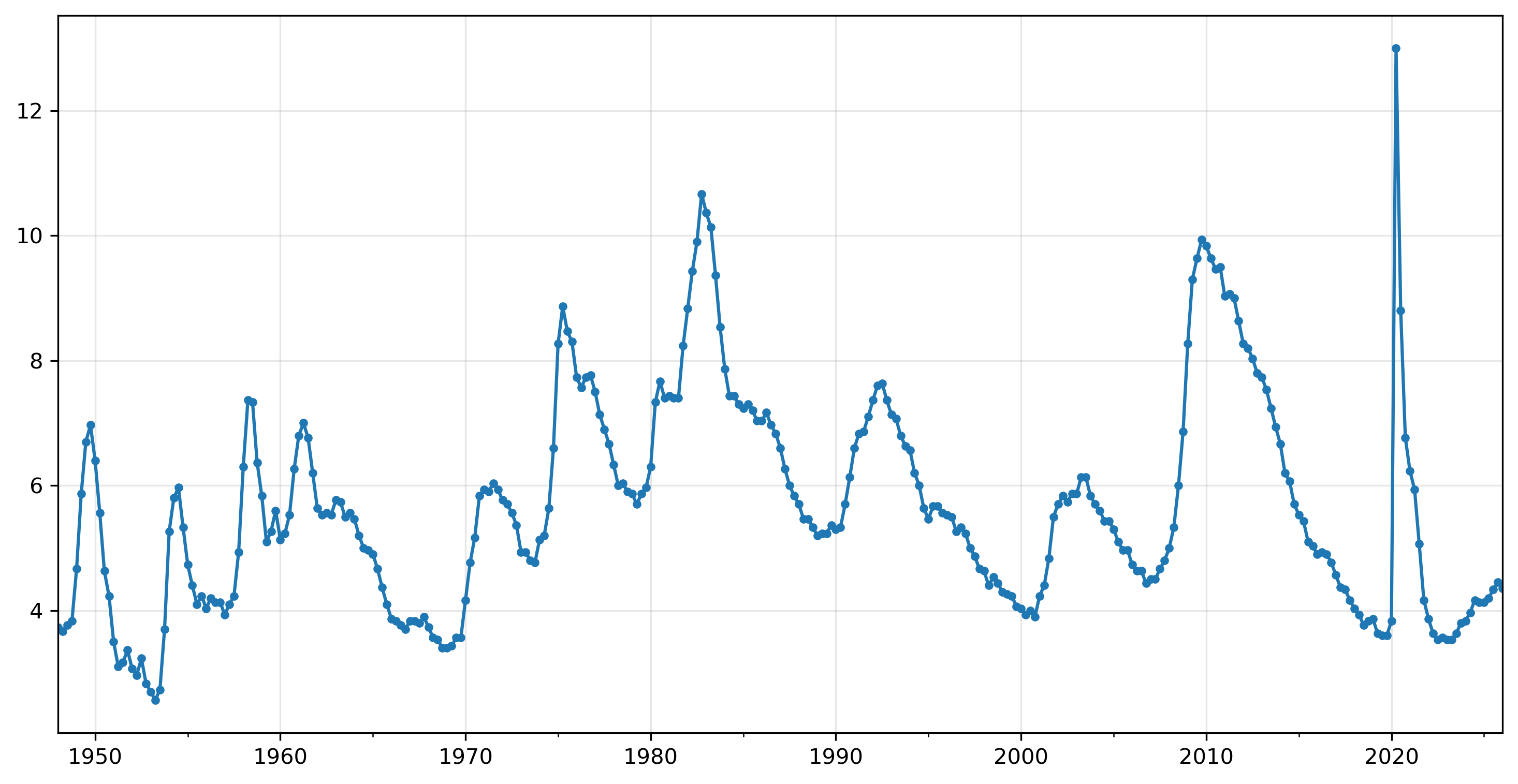
This application follows example in Tsay (2018), chapter 1. We’ll begin by downloading monthly unemployment data. This series, calculated by the Bureau of Labor Statistics, is seasonally adjusted and begins in 1948.
ur = pdr.get_data_fred('UNRATE', 1948)
We’ll begin by calculating the average rate on a quarterly basis. This is simple to do using the resample method in pandas, which is possible since we have a DatetimeIndex.
ur.index
DatetimeIndex(['1948-01-01', '1948-02-01', '1948-03-01', '1948-04-01',
               '1948-05-01', '1948-06-01', '1948-07-01', '1948-08-01',
               '1948-09-01', '1948-10-01',
               ...
               '2025-05-01', '2025-06-01', '2025-07-01', '2025-08-01',
               '2025-09-01', '2025-10-01', '2025-11-01', '2025-12-01',
               '2026-01-01', '2026-02-01'],
              dtype='datetime64[ns]', name='DATE', length=938, freq=None)
urq = ur.resample('Q')['UNRATE'].mean()
urq
DATE
1948-03-31    3.733333
1948-06-30    3.666667
1948-09-30    3.766667
1948-12-31    3.833333
1949-03-31    4.666667
                ...
2025-03-31    4.133333
2025-06-30    4.200000
2025-09-30    4.333333
2025-12-31    4.450000
2026-03-31    4.350000
Freq: QE-DEC, Name: UNRATE, Length: 313, dtype: float64
urq.plot(marker='.', xlabel='', grid=True);
urqd = urq.diff().dropna()
urqd.plot(marker='.', grid=True);
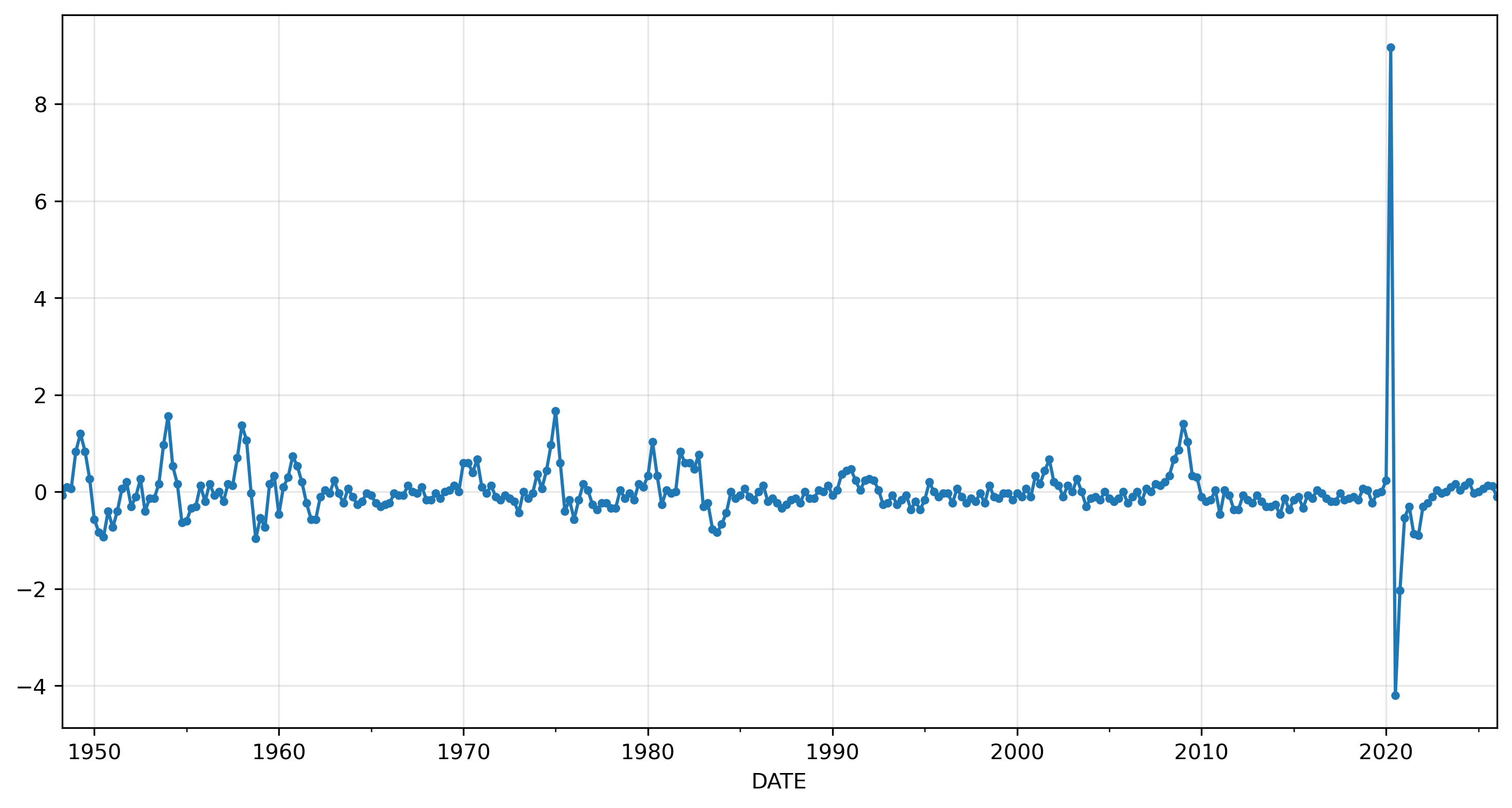
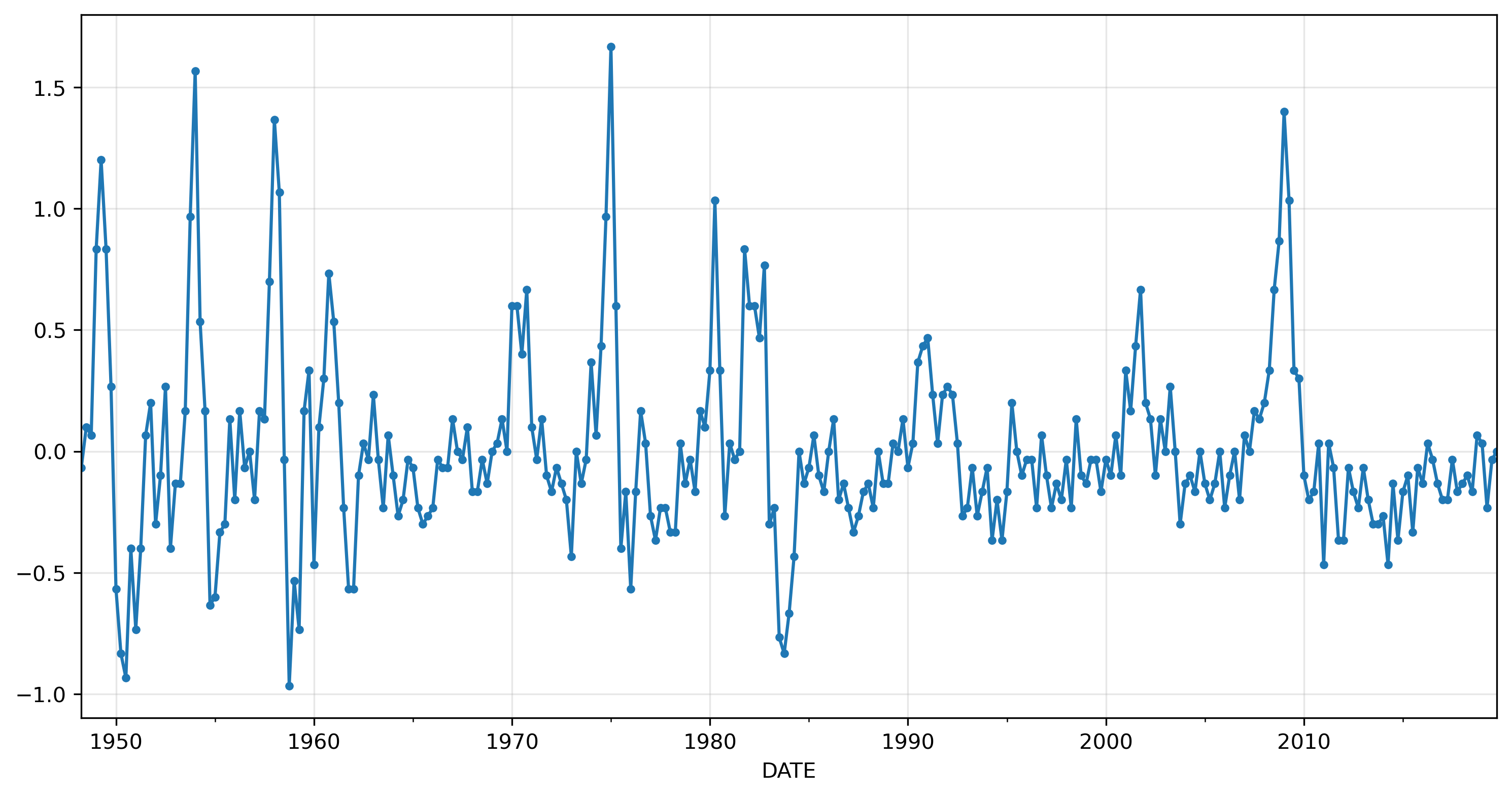
To simplify the analysis, we’ll drop the period at the end of the sample, when the pandemic caused a massive, never-before-seen change in unemployment.
urqd = urqd.loc[:'2019']

urqd.plot(marker='.', grid=True);
Model selection#
modsel = ar_select_order(urqd, maxlag=18, old_names=False)
# pass modsel.aic to pd.Series to get a nice table of AIC values

pd.Series(modsel.aic).round(4)
(1, 2, 3, 4, 5, 6, 7, 8, 9, 10, 11, 12, 13)                         54.3214
(1, 2, 3, 4, 5, 6, 7, 8, 9, 10, 11, 12)                             54.4209
(1, 2, 3, 4, 5, 6, 7, 8, 9, 10, 11, 12, 13, 14)                     55.8434
(1, 2, 3, 4, 5, 6, 7, 8, 9, 10, 11, 12, 13, 14, 15, 16, 17)         57.2608
(1, 2, 3, 4, 5, 6, 7, 8, 9, 10, 11, 12, 13, 14, 15, 16, 17, 18)     57.6978
(1, 2, 3, 4, 5, 6, 7, 8, 9, 10, 11, 12, 13, 14, 15)                 57.7964
(1, 2, 3, 4, 5, 6, 7, 8, 9, 10, 11, 12, 13, 14, 15, 16)             59.4825
(1, 2, 3, 4, 5, 6, 7, 8, 9, 10, 11)                                 61.8631
(1, 2, 3, 4, 5, 6, 7, 8, 9)                                         63.4146
(1, 2, 3, 4, 5, 6, 7, 8, 9, 10)                                     65.3997
(1, 2, 3, 4, 5, 6, 7, 8)                                            71.0780
(1, 2, 3, 4, 5, 6, 7)                                               77.3457
(1, 2, 3, 4, 5)                                                     77.6608
(1, 2, 3, 4)                                                        78.0792
(1, 2, 3, 4, 5, 6)                                                  78.5765
(1, 2, 3)                                                           79.5936
(1, 2)                                                              81.4666
(1,)                                                                84.6806
0                                                                  222.6336
dtype: float64
pd.Series(modsel.bic).round(4)
(1,)                                                                91.8701
(1, 2)                                                              92.2507
(1, 2, 3)                                                           93.9724
(1, 2, 3, 4)                                                        96.0527
(1, 2, 3, 4, 5)                                                     99.2291
(1, 2, 3, 4, 5, 6, 7, 8, 9)                                         99.3617
(1, 2, 3, 4, 5, 6, 7, 8, 9, 10, 11, 12)                            101.1522
(1, 2, 3, 4, 5, 6, 7, 8)                                           103.4304
(1, 2, 3, 4, 5, 6)                                                 103.7395
(1, 2, 3, 4, 5, 6, 7, 8, 9, 10, 11, 12, 13)                        104.6474
(1, 2, 3, 4, 5, 6, 7, 8, 9, 10)                                    104.9415
(1, 2, 3, 4, 5, 6, 7, 8, 9, 10, 11)                                104.9996
(1, 2, 3, 4, 5, 6, 7)                                              106.1034
(1, 2, 3, 4, 5, 6, 7, 8, 9, 10, 11, 12, 13, 14)                    109.7641
(1, 2, 3, 4, 5, 6, 7, 8, 9, 10, 11, 12, 13, 14, 15)                115.3118
(1, 2, 3, 4, 5, 6, 7, 8, 9, 10, 11, 12, 13, 14, 15, 16)            120.5926
(1, 2, 3, 4, 5, 6, 7, 8, 9, 10, 11, 12, 13, 14, 15, 16, 17)        121.9656
(1, 2, 3, 4, 5, 6, 7, 8, 9, 10, 11, 12, 13, 14, 15, 16, 17, 18)    125.9974
0                                                                  226.2283
dtype: float64
ar_select_order(urqd, maxlag=18, old_names=False, ic='aic').ar_lags
[1, 2, 3, 4, 5, 6, 7, 8, 9, 10, 11, 12, 13]
ar_select_order(urqd, maxlag=18, old_names=False, ic='bic').ar_lags
[1]
Using BIC would choose \(p=1\), but AIC indicates \(p=13\).
Comparing these two models using both AIC and BIC suggests \(p=13\) is a good model.
ar1 = AutoReg(urqd, lags=1).fit()
print(ar1.summary())
                            AutoReg Model Results
==============================================================================
Dep. Variable:                 UNRATE   No. Observations:                  287
Model:                     AutoReg(1)   Log Likelihood                 -51.751
Method:               Conditional MLE   S.D. of innovations              0.290
Date:                Mon, 30 Mar 2026   AIC                            109.501
Time:                        11:27:01   BIC                            120.469
Sample:                    09-30-1948   HQIC                           113.898
                         - 12-31-2019
==============================================================================
                 coef    std err          z      P>|z|      [0.025      0.975]
------------------------------------------------------------------------------
const       6.993e-05      0.017      0.004      0.997      -0.034       0.034
UNRATE.L1      0.6500      0.045     14.466      0.000       0.562       0.738
                                    Roots
=============================================================================
                  Real          Imaginary           Modulus         Frequency
-----------------------------------------------------------------------------
AR.1            1.5385           +0.0000j            1.5385            0.0000
-----------------------------------------------------------------------------
ar13 = AutoReg(urqd, lags=13).fit()
print(ar13.summary())
                            AutoReg Model Results
==============================================================================
Dep. Variable:                 UNRATE   No. Observations:                  287
Model:                    AutoReg(13)   Log Likelihood                 -16.418
Method:               Conditional MLE   S.D. of innovations              0.257
Date:                Mon, 30 Mar 2026   AIC                             62.836
Time:                        11:27:05   BIC                            117.033
Sample:                    09-30-1951   HQIC                            84.590
                         - 12-31-2019
==============================================================================
                 coef    std err          z      P>|z|      [0.025      0.975]
------------------------------------------------------------------------------
const          0.0010      0.016      0.061      0.951      -0.029       0.031
UNRATE.L1      0.7109      0.060     11.827      0.000       0.593       0.829
UNRATE.L2     -0.0097      0.072     -0.135      0.893      -0.151       0.132
UNRATE.L3     -0.0635      0.072     -0.881      0.378      -0.205       0.078
UNRATE.L4     -0.2520      0.072     -3.506      0.000      -0.393      -0.111
UNRATE.L5      0.0935      0.072      1.290      0.197      -0.049       0.235
UNRATE.L6      0.1542      0.069      2.220      0.026       0.018       0.290
UNRATE.L7      0.0011      0.070      0.016      0.987      -0.136       0.138
UNRATE.L8     -0.3298      0.069     -4.751      0.000      -0.466      -0.194
UNRATE.L9      0.1800      0.072      2.509      0.012       0.039       0.321
UNRATE.L10     0.0809      0.071      1.136      0.256      -0.059       0.220
UNRATE.L11    -0.0135      0.071     -0.190      0.849      -0.153       0.126
UNRATE.L12    -0.2278      0.071     -3.209      0.001      -0.367      -0.089
UNRATE.L13     0.0949      0.058      1.639      0.101      -0.019       0.208
                                    Roots
==============================================================================
                   Real          Imaginary           Modulus         Frequency
------------------------------------------------------------------------------
AR.1            -1.0734           -0.3600j            1.1321           -0.4485
AR.2            -1.0734           +0.3600j            1.1321            0.4485
AR.3            -0.8641           -0.8669j            1.2240           -0.3747
AR.4            -0.8641           +0.8669j            1.2240            0.3747
AR.5            -0.3644           -1.0261j            1.0889           -0.3043
AR.6            -0.3644           +1.0261j            1.0889            0.3043
AR.7             0.4348           -1.0201j            1.1089           -0.1859
AR.8             0.4348           +1.0201j            1.1089            0.1859
AR.9             0.8500           -0.7549j            1.1369           -0.1156
AR.10            0.8500           +0.7549j            1.1369            0.1156
AR.11            1.0908           -0.3209j            1.1371           -0.0455
AR.12            1.0908           +0.3209j            1.1371            0.0455
AR.13            2.2514           -0.0000j            2.2514           -0.0000
------------------------------------------------------------------------------
Let’s prune the model to keep only coefficients that are statistically significant.
ar13.tvalues
const          0.061384
UNRATE.L1     11.827093
UNRATE.L2     -0.134720
UNRATE.L3     -0.881150
UNRATE.L4     -3.506309
UNRATE.L5      1.289900
UNRATE.L6      2.220079
UNRATE.L7      0.016272
UNRATE.L8     -4.750995
UNRATE.L9      2.509202
UNRATE.L10     1.136459
UNRATE.L11    -0.190377
UNRATE.L12    -3.208969
UNRATE.L13     1.639165
dtype: float64
# 5% significance level

ar13.tvalues[ar13.tvalues.abs() > 1.96]
UNRATE.L1     11.827093
UNRATE.L4     -3.506309
UNRATE.L6      2.220079
UNRATE.L8     -4.750995
UNRATE.L9      2.509202
UNRATE.L12    -3.208969
dtype: float64
# 1% significance level

ar13.pvalues[ar13.pvalues < 0.01]
UNRATE.L1     2.827644e-32
UNRATE.L4     4.543675e-04
UNRATE.L8     2.024185e-06
UNRATE.L12    1.332118e-03
dtype: float64
ar_v2 = AutoReg(urqd, lags=[1, 4, 8, 12]).fit()

print(ar_v2.summary())
                            AutoReg Model Results
==============================================================================
Dep. Variable:                 UNRATE   No. Observations:                  287
Model:             Restr. AutoReg(12)   Log Likelihood                 -29.081
Method:               Conditional MLE   S.D. of innovations              0.269
Date:                Mon, 30 Mar 2026   AIC                             70.161
Time:                        11:27:09   BIC                             91.862
Sample:                    06-30-1951   HQIC                            78.870
                         - 12-31-2019
==============================================================================
                 coef    std err          z      P>|z|      [0.025      0.975]
------------------------------------------------------------------------------
const          0.0004      0.016      0.025      0.980      -0.031       0.032
UNRATE.L1      0.6276      0.045     14.010      0.000       0.540       0.715
UNRATE.L4     -0.1772      0.044     -3.987      0.000      -0.264      -0.090
UNRATE.L8     -0.1174      0.043     -2.733      0.006      -0.202      -0.033
UNRATE.L12    -0.1222      0.043     -2.856      0.004      -0.206      -0.038
                                    Roots
==============================================================================
                   Real          Imaginary           Modulus         Frequency
------------------------------------------------------------------------------
AR.1             1.0301           -0.3268j            1.0807           -0.0489
AR.2             1.0301           +0.3268j            1.0807            0.0489
AR.3             0.8843           -0.7578j            1.1645           -0.1128
AR.4             0.8843           +0.7578j            1.1645            0.1128
AR.5             0.4442           -1.1222j            1.2069           -0.1900
AR.6             0.4442           +1.1222j            1.2069            0.1900
AR.7            -0.3140           -1.1605j            1.2023           -0.2921
AR.8            -0.3140           +1.1605j            1.2023            0.2921
AR.9            -1.1815           -0.3878j            1.2435           -0.4495
AR.10           -1.1815           +0.3878j            1.2435            0.4495
AR.11           -0.8630           -0.9177j            1.2597           -0.3701
AR.12           -0.8630           +0.9177j            1.2597            0.3701
------------------------------------------------------------------------------
print(AutoReg(urqd, lags=[1, 4, 6, 8, 9, 12], trend='n').fit().summary())
                            AutoReg Model Results
==============================================================================
Dep. Variable:                 UNRATE   No. Observations:                  287
Model:             Restr. AutoReg(12)   Log Likelihood                 -19.055
Method:               Conditional MLE   S.D. of innovations              0.259
Date:                Mon, 30 Mar 2026   AIC                             52.110
Time:                        11:27:10   BIC                             77.427
Sample:                    06-30-1951   HQIC                            62.270
                         - 12-31-2019
==============================================================================
                 coef    std err          z      P>|z|      [0.025      0.975]
------------------------------------------------------------------------------
UNRATE.L1      0.6668      0.044     15.141      0.000       0.580       0.753
UNRATE.L4     -0.2399      0.047     -5.126      0.000      -0.332      -0.148
UNRATE.L6      0.1848      0.049      3.745      0.000       0.088       0.282
UNRATE.L8     -0.3058      0.061     -5.047      0.000      -0.425      -0.187
UNRATE.L9      0.1861      0.056      3.323      0.001       0.076       0.296
UNRATE.L12    -0.1472      0.042     -3.512      0.000      -0.229      -0.065
                                    Roots
==============================================================================
                   Real          Imaginary           Modulus         Frequency
------------------------------------------------------------------------------
AR.1             1.0569           -0.2923j            1.0966           -0.0429
AR.2             1.0569           +0.2923j            1.0966            0.0429
AR.3             0.8633           -0.7253j            1.1275           -0.1112
AR.4             0.8633           +0.7253j            1.1275            0.1112
AR.5             0.4598           -1.0438j            1.1406           -0.1840
AR.6             0.4598           +1.0438j            1.1406            0.1840
AR.7            -1.0861           -0.3895j            1.1538           -0.4452
AR.8            -1.0861           +0.3895j            1.1538            0.4452
AR.9            -0.4159           -1.0497j            1.1290           -0.3100
AR.10           -0.4159           +1.0497j            1.1290            0.3100
AR.11           -0.8780           -1.1148j            1.4190           -0.3562
AR.12           -0.8780           +1.1148j            1.4190            0.3562
------------------------------------------------------------------------------
Using glob=True performs a global search over all \(2^{12}=4096\) possible models. Clearly trying all possible models for a large number of lags would eventually become infeasible; using 20 lags requires testing over 1 million models, for example.
sel = ar_select_order(urqd, 12, old_names=False, glob=True)
sel.ar_lags
[1, 4, 6, 8, 9, 12]
Residuals#
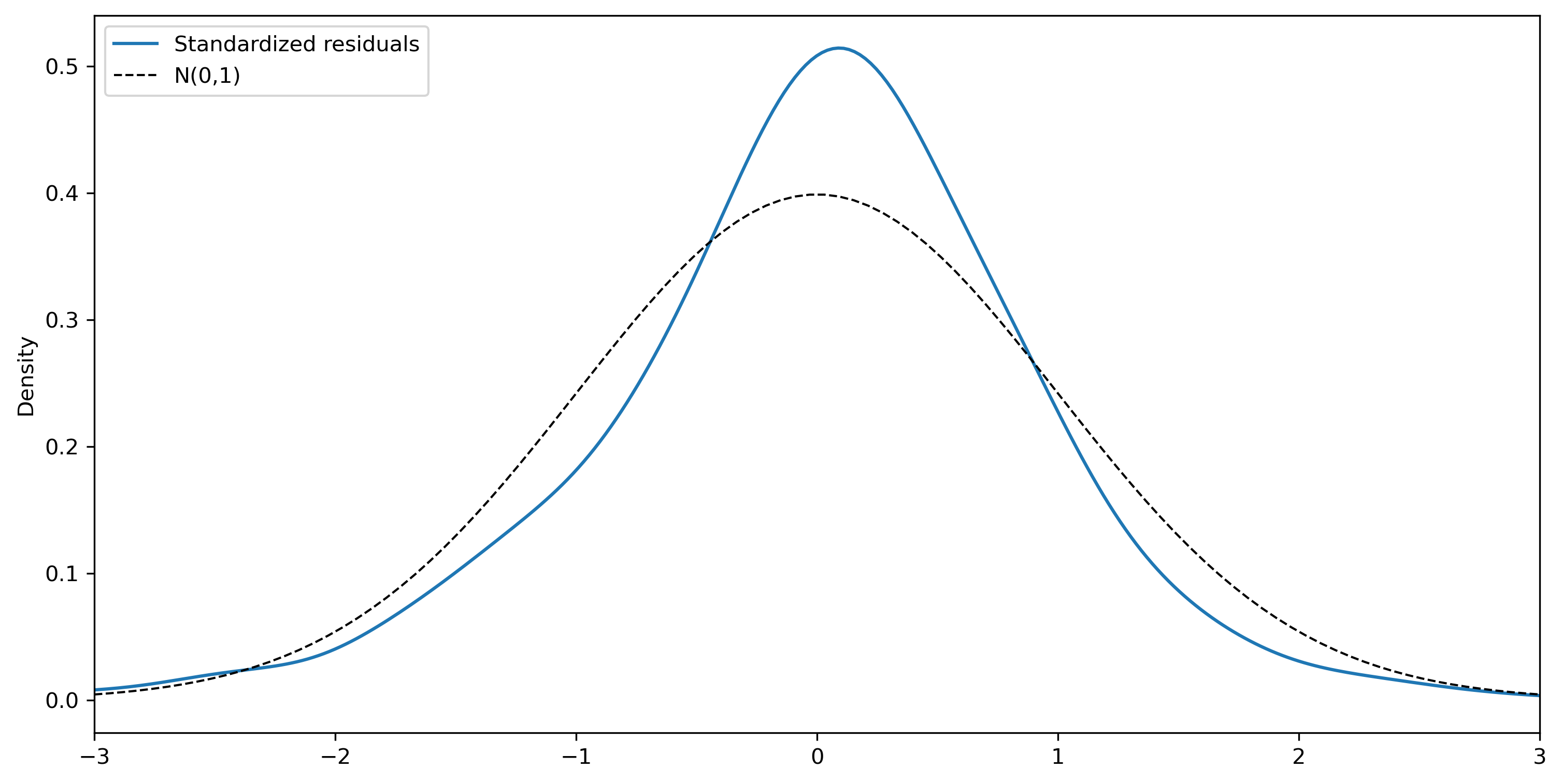
The standardized residuals are calculated by scaling the residuals from their estimated standard deviation, \(\epsilon_t / \sigma.\)
std_resid = ar_v2.resid / np.sqrt(ar_v2.sigma2)
We can use kernel density estimation to get an empirical estimate of the PDF.
ax = std_resid.plot.kde(xlim=(-3,3), bw_method=0.25)
ax.grid(alpha=0.25)
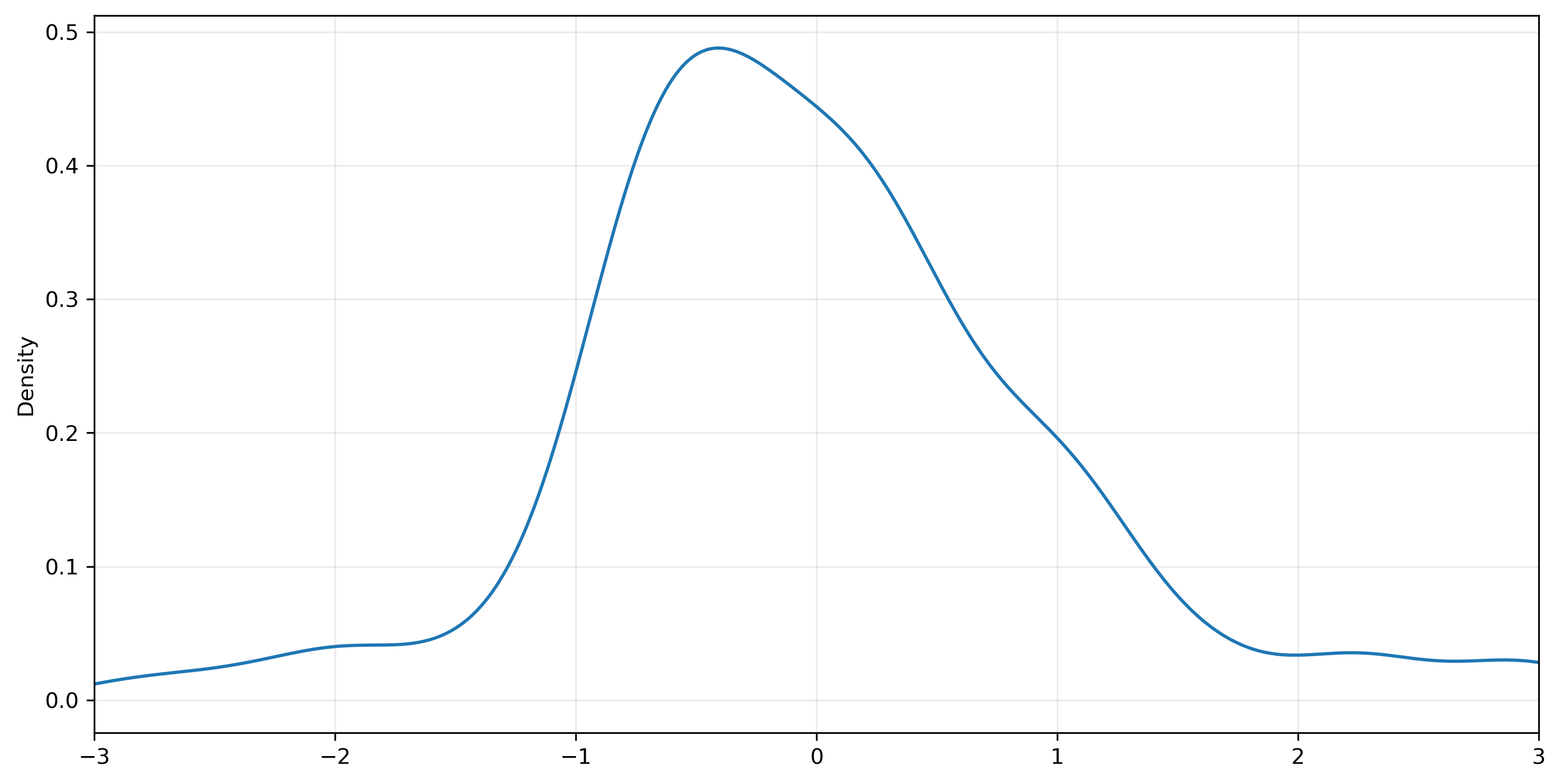
std_resid.skew(), std_resid.kurtosis()
(0.5712214353027926, 1.8777501533375105)
There are several statistical tests we can use to test the null hypothesis that data are drawn from a normal distribution. Two that are available in scipy are due to D’Agostino and Pearson (1973) and the Shapiro and Wilk (1965). The former combines information about the skewness and kurtosis of a series; the latter is a more complicated test that uses information about order statistics.
from scipy.stats import normaltest, shapiro
normaltest(std_resid)
NormaltestResult(statistic=28.285962906502313, pvalue=7.207442680254298e-07)
shapiro(std_resid)
ShapiroResult(statistic=0.958171619651281, pvalue=4.0510448979408166e-07)
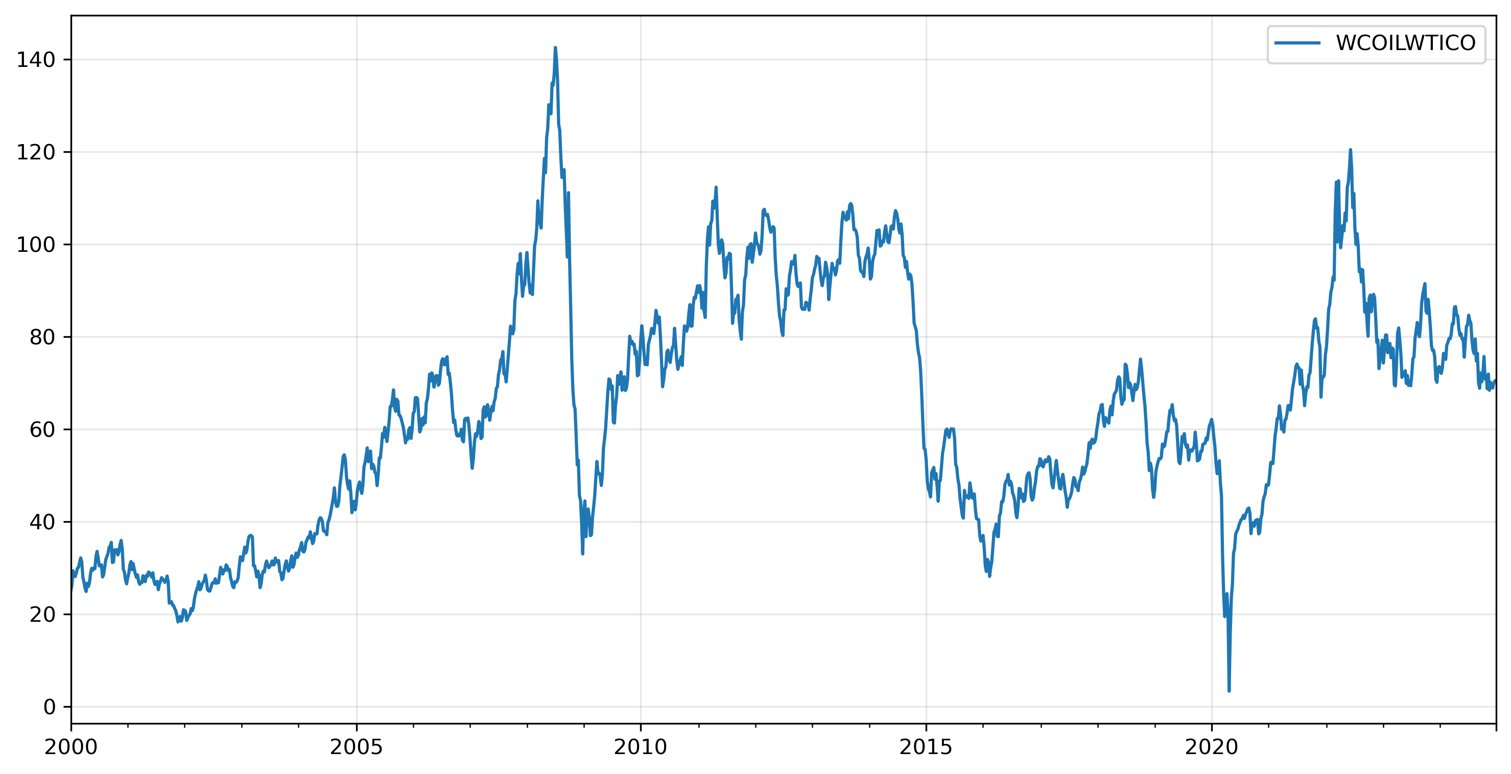
Oil prices#
Next we’ll use the Crude Oil Price series for West Texas Intermediate at Cushing, Oklahoma (WTI), available from FRED.
oil = pdr.get_data_fred('WCOILWTICO', 2000, 2025)
oil.index
DatetimeIndex(['2000-01-07', '2000-01-14', '2000-01-21', '2000-01-28',
               '2000-02-04', '2000-02-11', '2000-02-18', '2000-02-25',
               '2000-03-03', '2000-03-10',
               ...
               '2024-10-25', '2024-11-01', '2024-11-08', '2024-11-15',
               '2024-11-22', '2024-11-29', '2024-12-06', '2024-12-13',
               '2024-12-20', '2024-12-27'],
              dtype='datetime64[ns]', name='DATE', length=1304, freq=None)
# specify a frequency for the series
oil.index = pd.DatetimeIndex(oil.index, freq='W-FRI')
ax = oil.plot(xlabel='')
ax.grid(alpha=0.3)
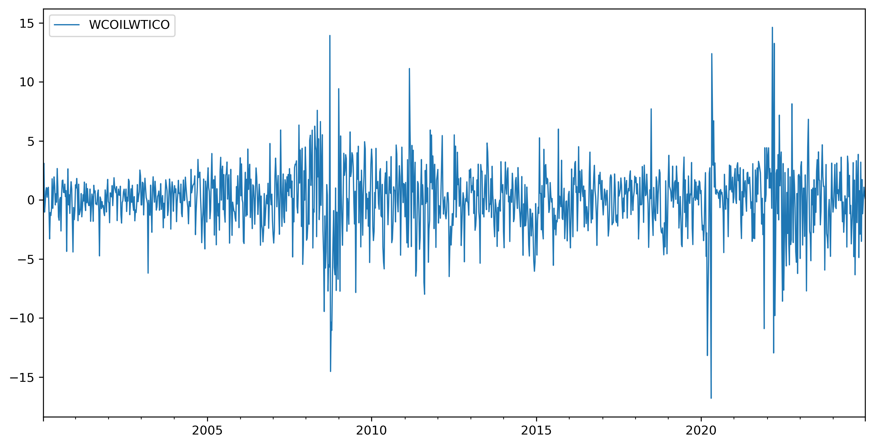
oild = oil.diff().dropna()
oild.plot(lw=1, xlabel='');
ar_select_order(oild, maxlag=18, old_names=False, ic='aic').ar_lags
[1, 2, 3, 4, 5, 6, 7, 8, 9, 10, 11, 12, 13, 14, 15, 16, 17]
ar = AutoReg(oild, lags=17, old_names=False).fit()
print(ar.summary())
                            AutoReg Model Results
==============================================================================
Dep. Variable:             WCOILWTICO   No. Observations:                 1303
Model:                    AutoReg(17)   Log Likelihood               -3096.451
Method:               Conditional MLE   S.D. of innovations              2.688
Date:                Mon, 30 Mar 2026   AIC                           6230.902
Time:                        12:10:56   BIC                           6328.929
Sample:                    05-12-2000   HQIC                          6267.702
                         - 12-27-2024
==================================================================================
                     coef    std err          z      P>|z|      [0.025      0.975]
----------------------------------------------------------------------------------
const              0.0246      0.075      0.329      0.743      -0.122       0.172
WCOILWTICO.L1      0.1428      0.028      5.128      0.000       0.088       0.197
WCOILWTICO.L2     -0.0012      0.028     -0.043      0.965      -0.056       0.054
WCOILWTICO.L3      0.0630      0.028      2.248      0.025       0.008       0.118
WCOILWTICO.L4     -0.0087      0.028     -0.308      0.758      -0.064       0.046
WCOILWTICO.L5      0.0439      0.028      1.569      0.117      -0.011       0.099
WCOILWTICO.L6      0.0337      0.028      1.200      0.230      -0.021       0.089
WCOILWTICO.L7     -0.0216      0.028     -0.770      0.441      -0.077       0.033
WCOILWTICO.L8      0.1108      0.028      3.942      0.000       0.056       0.166
WCOILWTICO.L9     -0.0605      0.028     -2.140      0.032      -0.116      -0.005
WCOILWTICO.L10     0.0056      0.028      0.199      0.842      -0.050       0.061
WCOILWTICO.L11    -0.0049      0.028     -0.173      0.862      -0.060       0.050
WCOILWTICO.L12     0.0184      0.028      0.654      0.513      -0.037       0.074
WCOILWTICO.L13    -0.0640      0.028     -2.272      0.023      -0.119      -0.009
WCOILWTICO.L14     0.0492      0.028      1.744      0.081      -0.006       0.105
WCOILWTICO.L15    -0.0174      0.028     -0.616      0.538      -0.073       0.038
WCOILWTICO.L16    -0.0737      0.028     -2.613      0.009      -0.129      -0.018
WCOILWTICO.L17     0.0593      0.028      2.116      0.034       0.004       0.114
                                    Roots
==============================================================================
                   Real          Imaginary           Modulus         Frequency
------------------------------------------------------------------------------
AR.1            -1.1847           -0.1382j            1.1927           -0.4815
AR.2            -1.1847           +0.1382j            1.1927            0.4815
AR.3            -0.9510           -0.6157j            1.1329           -0.4086
AR.4            -0.9510           +0.6157j            1.1329            0.4086
AR.5            -0.6576           -0.8816j            1.0998           -0.3520
AR.6            -0.6576           +0.8816j            1.0998            0.3520
AR.7            -0.2201           -1.1087j            1.1303           -0.2812
AR.8            -0.2201           +1.1087j            1.1303            0.2812
AR.9             0.1814           -1.1568j            1.1709           -0.2252
AR.10            0.1814           +1.1568j            1.1709            0.2252
AR.11            0.6172           -1.0118j            1.1852           -0.1628
AR.12            0.6172           +1.0118j            1.1852            0.1628
AR.13            0.9385           -0.7602j            1.2078           -0.1084
AR.14            0.9385           +0.7602j            1.2078            0.1084
AR.15            1.2165           -0.2853j            1.2495           -0.0367
AR.16            1.2165           +0.2853j            1.2495            0.0367
AR.17            1.3631           -0.0000j            1.3631           -0.0000
------------------------------------------------------------------------------
# 1% significance level

ar.tvalues[ar.tvalues.abs() > 2.326]
WCOILWTICO.L1     5.128402
WCOILWTICO.L8     3.942358
WCOILWTICO.L16   -2.613228
dtype: float64
ar_b = AutoReg(oild, lags=[1,8,16], old_names=False).fit()
print(ar_b.summary())
                            AutoReg Model Results
==============================================================================
Dep. Variable:             WCOILWTICO   No. Observations:                 1303
Model:             Restr. AutoReg(16)   Log Likelihood               -3111.642
Method:               Conditional MLE   S.D. of innovations              2.715
Date:                Mon, 30 Mar 2026   AIC                           6233.284
Time:                        12:12:39   BIC                           6259.085
Sample:                    05-05-2000   HQIC                          6242.970
                         - 12-27-2024
==================================================================================
                     coef    std err          z      P>|z|      [0.025      0.975]
----------------------------------------------------------------------------------
const              0.0296      0.076      0.392      0.695      -0.119       0.178
WCOILWTICO.L1      0.1317      0.027      4.803      0.000       0.078       0.185
WCOILWTICO.L8      0.1056      0.028      3.829      0.000       0.052       0.160
WCOILWTICO.L16    -0.0735      0.028     -2.659      0.008      -0.128      -0.019
                                    Roots
==============================================================================
                   Real          Imaginary           Modulus         Frequency
------------------------------------------------------------------------------
AR.1             1.1493           -0.1948j            1.1657           -0.0267
AR.2             1.1493           +0.1948j            1.1657            0.0267
AR.3             0.9566           -0.6670j            1.1662           -0.0969
AR.4             0.9566           +0.6670j            1.1662            0.0969
AR.5             0.6846           -0.9526j            1.1730           -0.1508
AR.6             0.6846           +0.9526j            1.1730            0.1508
AR.7             0.2118           -1.1545j            1.1737           -0.2211
AR.8             0.2118           +1.1545j            1.1737            0.2211
AR.9            -0.1919           -1.1663j            1.1820           -0.2760
AR.10           -0.1919           +1.1663j            1.1820            0.2760
AR.11           -0.6725           -0.9724j            1.1823           -0.3463
AR.12           -0.6725           +0.9724j            1.1823            0.3463
AR.13           -0.9684           -0.6871j            1.1874           -0.4018
AR.14           -0.9684           +0.6871j            1.1874            0.4018
AR.15           -1.1693           -0.2068j            1.1875           -0.4721
AR.16           -1.1693           +0.2068j            1.1875            0.4721
------------------------------------------------------------------------------
std_resid = ar_b.resid / np.sqrt(ar_b.sigma2)
std_resid.skew(), std_resid.kurtosis()
(-0.2535073744148516, 5.4491566084082415)
normaltest(std_resid)
NormaltestResult(statistic=171.8329216954173, pvalue=4.863569756405212e-38)
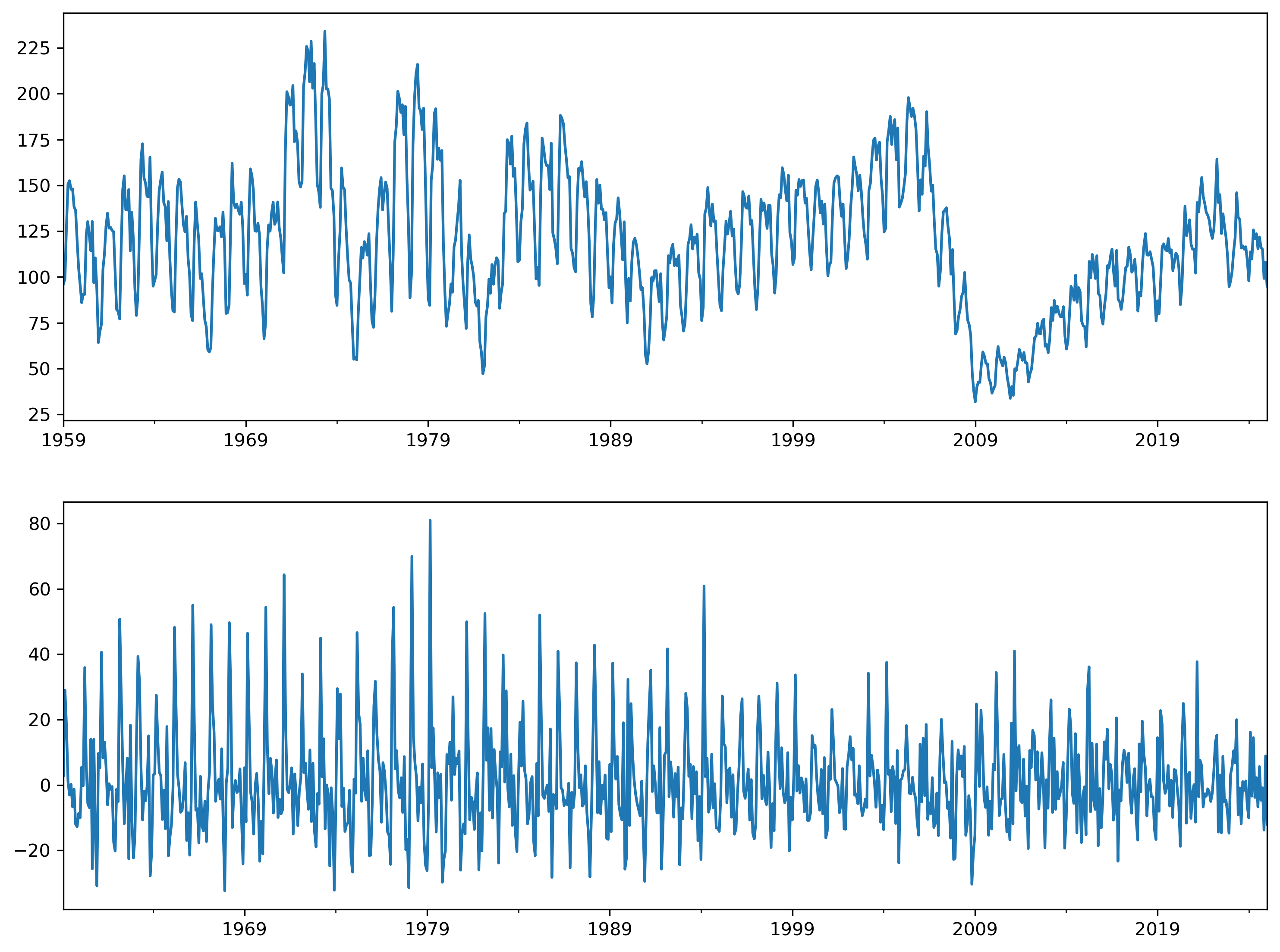
Housing starts#
Next we’ll examine housing starts using the series Housing Starts: Total: New Privately Owned Housing Units Started (HOUSTNSA).
hstarts = pdr.get_data_fred('HOUSTNSA', 1959, 2025).asfreq('MS').squeeze()
sel = ar_select_order(hstartsd, 24, old_names=False)

# fit selected model
res = sel.model.fit()

print(res.summary())
                            AutoReg Model Results
==============================================================================
Dep. Variable:               HOUSTNSA   No. Observations:                  792
Model:                    AutoReg(24)   Log Likelihood               -2848.436
Method:               Conditional MLE   S.D. of innovations              9.875
Date:                Mon, 30 Mar 2026   AIC                           5748.872
Time:                        12:15:21   BIC                           5869.610
Sample:                    02-01-1961   HQIC                          5795.343
                         - 01-01-2025
================================================================================
                   coef    std err          z      P>|z|      [0.025      0.975]
--------------------------------------------------------------------------------
const            1.5393      0.461      3.341      0.001       0.636       2.442
HOUSTNSA.L1     -0.2832      0.035     -8.062      0.000      -0.352      -0.214
HOUSTNSA.L2     -0.1187      0.036     -3.254      0.001      -0.190      -0.047
HOUSTNSA.L3     -0.0450      0.037     -1.225      0.220      -0.117       0.027
HOUSTNSA.L4     -0.0753      0.037     -2.057      0.040      -0.147      -0.004
HOUSTNSA.L5     -0.0107      0.036     -0.293      0.769      -0.082       0.061
HOUSTNSA.L6     -0.0470      0.036     -1.289      0.197      -0.119       0.024
HOUSTNSA.L7     -0.0481      0.036     -1.321      0.186      -0.119       0.023
HOUSTNSA.L8     -0.0775      0.036     -2.130      0.033      -0.149      -0.006
HOUSTNSA.L9     -0.0279      0.036     -0.769      0.442      -0.099       0.043
HOUSTNSA.L10    -0.1118      0.036     -3.087      0.002      -0.183      -0.041
HOUSTNSA.L11     0.0277      0.036      0.762      0.446      -0.044       0.099
HOUSTNSA.L12     0.3472      0.035      9.879      0.000       0.278       0.416
HOUSTNSA.L13     0.2475      0.035      7.042      0.000       0.179       0.316
HOUSTNSA.L14     0.0466      0.036      1.287      0.198      -0.024       0.118
HOUSTNSA.L15    -0.0273      0.036     -0.757      0.449      -0.098       0.043
HOUSTNSA.L16    -0.1371      0.036     -3.803      0.000      -0.208      -0.066
HOUSTNSA.L17    -0.0259      0.036     -0.714      0.475      -0.097       0.045
HOUSTNSA.L18    -0.0848      0.036     -2.340      0.019      -0.156      -0.014
HOUSTNSA.L19     0.0015      0.036      0.042      0.966      -0.070       0.073
HOUSTNSA.L20    -0.0930      0.036     -2.559      0.010      -0.164      -0.022
HOUSTNSA.L21    -0.0929      0.036     -2.553      0.011      -0.164      -0.022
HOUSTNSA.L22    -0.0094      0.037     -0.258      0.797      -0.081       0.062
HOUSTNSA.L23     0.0607      0.036      1.675      0.094      -0.010       0.132
HOUSTNSA.L24     0.2272      0.035      6.525      0.000       0.159       0.295
                                    Roots
==============================================================================
                   Real          Imaginary           Modulus         Frequency
------------------------------------------------------------------------------
AR.1            -1.1039           -0.0000j            1.1039           -0.5000
AR.2            -1.0266           -0.2516j            1.0570           -0.4617
AR.3            -1.0266           +0.2516j            1.0570            0.4617
AR.4            -0.8897           -0.5143j            1.0276           -0.4166
AR.5            -0.8897           +0.5143j            1.0276            0.4166
AR.6            -0.7635           -0.7742j            1.0874           -0.3739
AR.7            -0.7635           +0.7742j            1.0874            0.3739
AR.8            -0.5372           -0.9002j            1.0483           -0.3356
AR.9            -0.5372           +0.9002j            1.0483            0.3356
AR.10           -0.3285           -1.0522j            1.1023           -0.2982
AR.11           -0.3285           +1.0522j            1.1023            0.2982
AR.12           -0.0143           -1.0421j            1.0422           -0.2522
AR.13           -0.0143           +1.0421j            1.0422            0.2522
AR.14            0.2139           -1.0530j            1.0745           -0.2181
AR.15            0.2139           +1.0530j            1.0745            0.2181
AR.16            0.5019           -0.8717j            1.0059           -0.1669
AR.17            0.5019           +0.8717j            1.0059            0.1669
AR.18            0.7584           -0.8062j            1.1068           -0.1299
AR.19            0.7584           +0.8062j            1.1068            0.1299
AR.20            0.8700           -0.5015j            1.0042           -0.0832
AR.21            0.8700           +0.5015j            1.0042            0.0832
AR.22            1.0827           -0.2575j            1.1129           -0.0372
AR.23            1.0827           +0.2575j            1.1129            0.0372
AR.24            1.1026           -0.0000j            1.1026           -0.0000
------------------------------------------------------------------------------
Removing seasonality#
By allowing each month of the year to have its own intercept — or “dummy variable” — we can remove the seasonal variation in the series.
hstartsd.groupby(hstartsd.index.month).mean()
DATE
1     -4.269131
2      4.160395
3     31.359965
4     13.224910
5      4.059291
6      0.538924
7     -3.537971
8     -1.794444
9     -4.022403
10     2.524579
11   -15.054469
12   -13.934532
Name: HOUSTNSA, dtype: float64
When estimating an autoregression or running order selection, we can include seasonal dummies. Here’s we’ll exclude the main intercept and instead have 12 dummies (one for each month).
sel = ar_select_order(hstartsd, 24, seasonal=True, trend='n', old_names=False)
sel.ar_lags
[1]
The initial data begin in January, but when we difference the data we end up with a series that starts in February. Therefore, the s(1,12) coefficient is automatically defined as the February dummy.
res = sel.model.fit()
print(res.summary())
                            AutoReg Model Results
==============================================================================
Dep. Variable:               HOUSTNSA   No. Observations:                  792
Model:               Seas. AutoReg(1)   Log Likelihood               -2932.672
Method:               Conditional MLE   S.D. of innovations              9.861
Date:                Mon, 30 Mar 2026   AIC                           5893.345
Time:                        12:15:36   BIC                           5958.771
Sample:                    03-01-1959   HQIC                          5918.492
                         - 01-01-2025
===============================================================================
                  coef    std err          z      P>|z|      [0.025      0.975]
-------------------------------------------------------------------------------
s(1,12)         3.2422      1.232      2.633      0.008       0.828       5.656
s(2,12)        32.2999      1.222     26.424      0.000      29.904      34.696
s(3,12)        20.3096      1.629     12.466      0.000      17.117      23.503
s(4,12)         7.0470      1.297      5.431      0.000       4.504       9.590
s(5,12)         1.4560      1.222      1.192      0.233      -0.939       3.851
s(6,12)        -3.4162      1.214     -2.814      0.005      -5.796      -1.037
s(7,12)        -2.5937      1.220     -2.126      0.034      -4.985      -0.203
s(8,12)        -4.4278      1.215     -3.643      0.000      -6.810      -2.046
s(9,12)         1.6159      1.222      1.323      0.186      -0.779       4.011
s(10,12)      -14.4841      1.217    -11.902      0.000     -16.869     -12.099
s(11,12)      -17.3356      1.321    -13.121      0.000     -19.925     -14.746
s(12,12)       -7.4172      1.306     -5.678      0.000      -9.978      -4.857
HOUSTNSA.L1    -0.2259      0.035     -6.520      0.000      -0.294      -0.158
                                    Roots
=============================================================================
                  Real          Imaginary           Modulus         Frequency
-----------------------------------------------------------------------------
AR.1           -4.4264           +0.0000j            4.4264            0.5000
-----------------------------------------------------------------------------
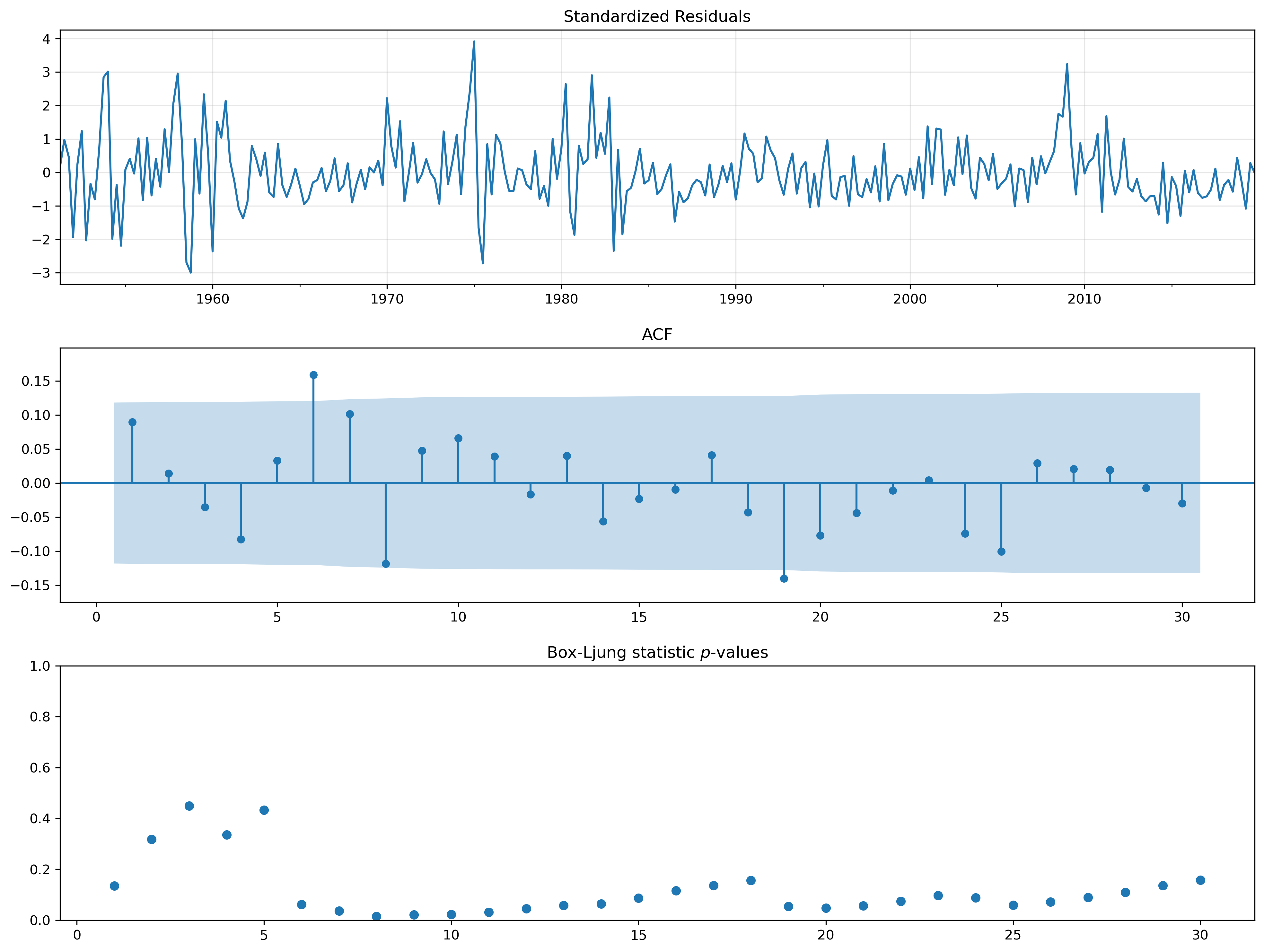
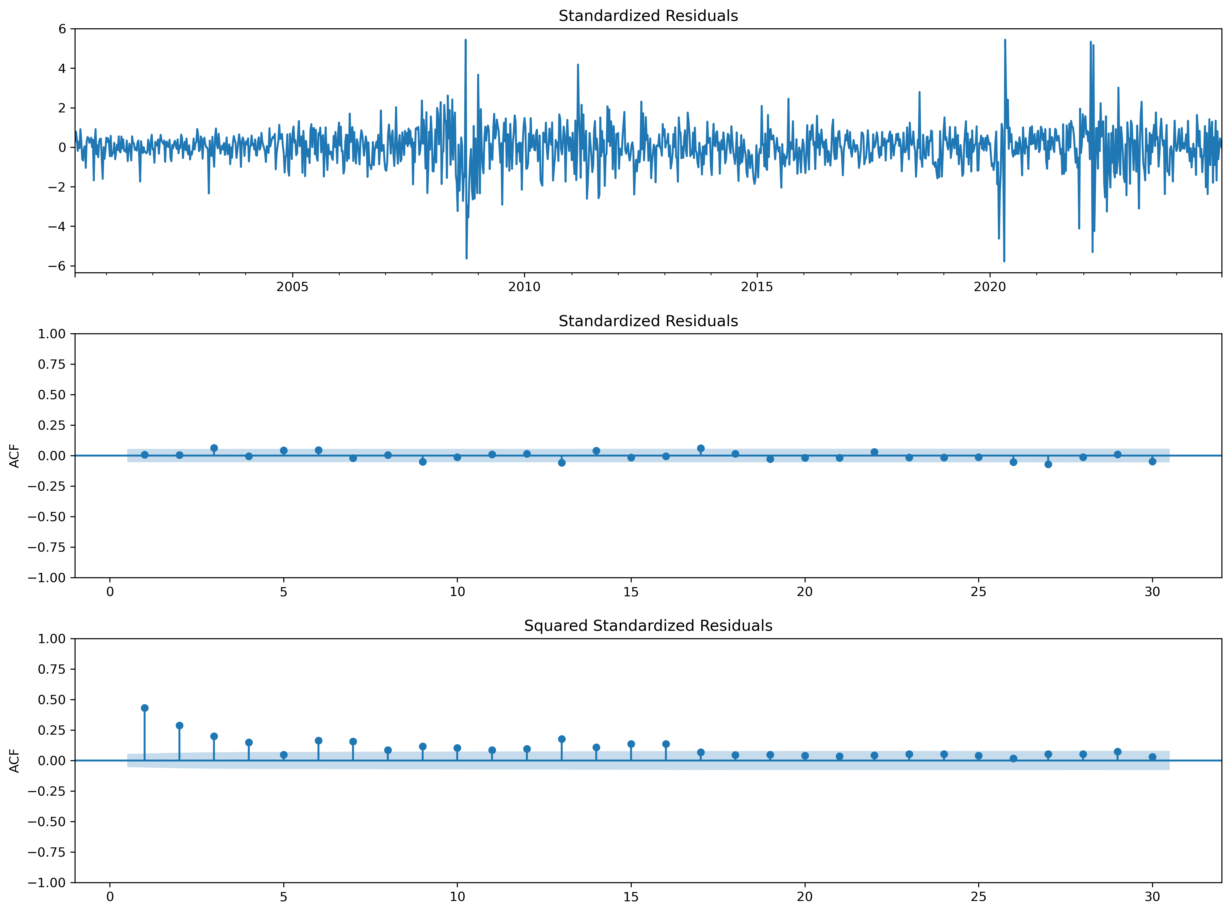
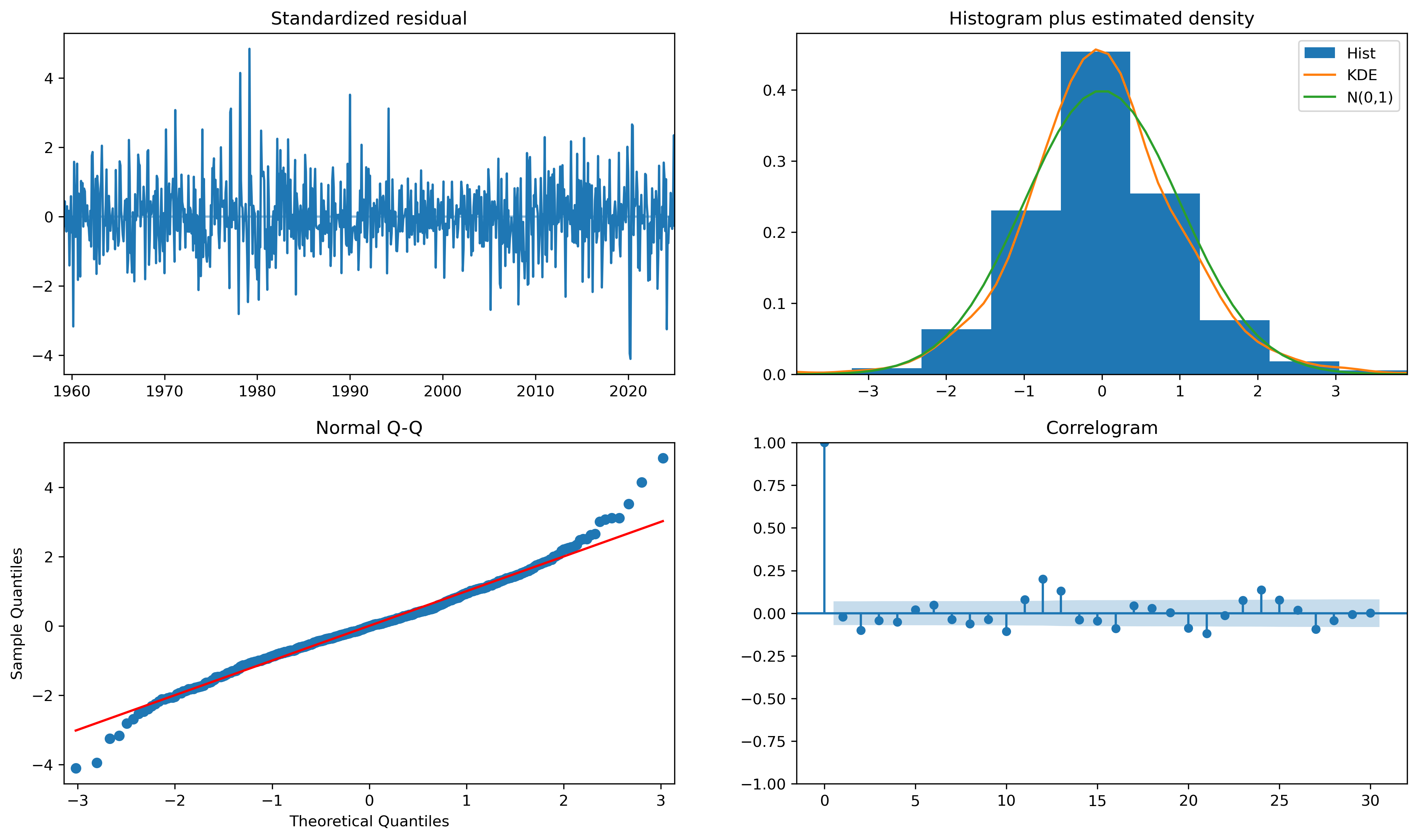
fig = plt.figure(figsize=(16,9))
fig = res.plot_diagnostics(fig=fig, lags=30)
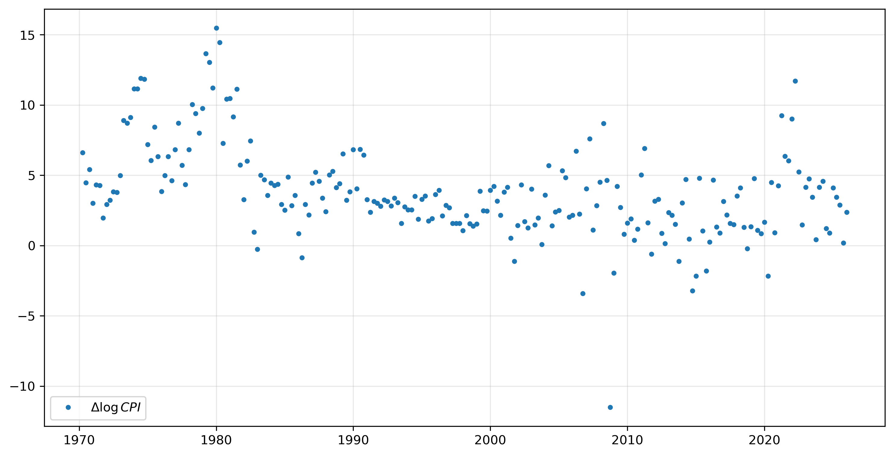
Inflation#
Consumer Price Index for All Urban Consumers: All Items in U.S. City Average (CPIAUCNS)
cpi = pdr.get_data_fred('CPIAUCNS', start=1970).squeeze()

cpi.index = pd.DatetimeIndex(cpi.index, freq='MS')
cpi.tail(10)
DATE
2025-05-01    321.465
2025-06-01    322.561
2025-07-01    323.048
2025-08-01    323.976
2025-09-01    324.800
2025-10-01        NaN
2025-11-01    324.122
2025-12-01    324.054
2026-01-01    325.252
2026-02-01    326.785
Freq: MS, Name: CPIAUCNS, dtype: float64
# calculating an annualized inflation rate in percent
inf = np.log(cpi).resample('QS').mean().diff()[1:] * 400
inf.tail(10)
DATE
2023-10-01    0.419097
2024-01-01    4.143722
2024-04-01    4.582997
2024-07-01    1.206464
2024-10-01    0.898997
2025-01-01    4.113436
2025-04-01    3.443490
2025-07-01    2.892898
2025-10-01    0.182036
2026-01-01    2.374514
Freq: QS-JAN, Name: CPIAUCNS, dtype: float64
Another flexible model for estimation are seasonal autoregressive integrated moving average models, or SARIMAX. These models are a class of state space models,
Here, we observe the time series \(y_t\), but it depends on the state variable, \(\alpha_{t}\), which is unobservable. The \(\varepsilon\) and \(\eta\) terms are both noise processes. (Uppercase letters denote matrices, while lowercase letters are vectors.) The first equation is called the observation equation while the second set of equations are the state equations.
This class of models nests ARMA models as well as other types of models. For example, we can write the ARMA(1,1) model
as a state-space model:
To see this, note that the observation equation says
which implies that
The two state equations imply that
and
Substituting these into (15), we get
which is the desired ARMA(1,1) model.
The following examples are based on those of Chad Fulton, an economist at the Federal Reserve.
# Estimate ARMA(1,1) model with SARIMAX
inf_model2 = sm.tsa.SARIMAX(inf, order=(1, 0, 1))
inf_results2 = inf_model2.fit()

print(inf_results2.summary())
RUNNING THE L-BFGS-B CODE

           * * *

Machine precision = 2.220D-16
 N =            3     M =           10

At X0         0 variables are exactly at the bounds

At iterate    0    f=  2.40150D+00    |proj g|=  1.02415D-01

At iterate    5    f=  2.36720D+00    |proj g|=  6.26196D-02

At iterate   10    f=  2.35807D+00    |proj g|=  1.00190D-03

At iterate   15    f=  2.35804D+00    |proj g|=  1.58860D-06

           * * *

Tit   = total number of iterations
Tnf   = total number of function evaluations
Tnint = total number of segments explored during Cauchy searches
Skip  = number of BFGS updates skipped
Nact  = number of active bounds at final generalized Cauchy point
Projg = norm of the final projected gradient
F     = final function value

           * * *

   N    Tit     Tnf  Tnint  Skip  Nact     Projg        F
    3     15     17      1     0     0   1.589D-06   2.358D+00
  F =   2.3580439428985573

CONVERGENCE: NORM_OF_PROJECTED_GRADIENT_<=_PGTOL
                               SARIMAX Results
==============================================================================
Dep. Variable:               CPIAUCNS   No. Observations:                  224
Model:               SARIMAX(1, 0, 1)   Log Likelihood                -528.202
Date:                Mon, 30 Mar 2026   AIC                           1062.404
Time:                        12:17:59   BIC                           1072.639
Sample:                    04-01-1970   HQIC                          1066.535
                         - 01-01-2026
Covariance Type:                  opg
==============================================================================
                 coef    std err          z      P>|z|      [0.025      0.975]
------------------------------------------------------------------------------
ar.L1          0.9771      0.015     64.390      0.000       0.947       1.007
ma.L1         -0.6176      0.056    -11.014      0.000      -0.727      -0.508
sigma2         6.4916      0.317     20.457      0.000       5.870       7.114
===================================================================================
Ljung-Box (L1) (Q):                   4.32   Jarque-Bera (JB):               558.70
Prob(Q):                              0.04   Prob(JB):                         0.00
Heteroskedasticity (H):               1.82   Skew:                            -1.17
Prob(H) (two-sided):                  0.01   Kurtosis:                        10.37
===================================================================================

Warnings:
[1] Covariance matrix calculated using the outer product of gradients (complex-step).
This problem is unconstrained.
Notice that the observation from October 2008 is quite different from all the other data. This outlier might be having a out-sized impact on our results, so we can remove its effect by letting it have its own intercept. We do this by including an additional exogenous variable in the regression using the exog argument; in this case the variable is a vector that is zero for every observation except the one for October 2008.
outlier = pd.Series(np.zeros(len(inf)), index=inf.index, name='outlier')
outlier['2008-10-01'] = 1
inf_model3 = sm.tsa.SARIMAX(inf, order=(1, 0, 1), exog=outlier)
inf_results3 = inf_model3.fit()

print(inf_results3.summary())
RUNNING THE L-BFGS-B CODE

           * * *

Machine precision = 2.220D-16
 N =            4     M =           10

At X0         0 variables are exactly at the bounds

At iterate    0    f=  2.30107D+00    |proj g|=  1.14907D-01

At iterate    5    f=  2.26805D+00    |proj g|=  3.18944D-02

At iterate   10    f=  2.26137D+00    |proj g|=  1.75196D-03

At iterate   15    f=  2.25957D+00    |proj g|=  1.20166D-03

           * * *

Tit   = total number of iterations
Tnf   = total number of function evaluations
Tnint = total number of segments explored during Cauchy searches
Skip  = number of BFGS updates skipped
Nact  = number of active bounds at final generalized Cauchy point
Projg = norm of the final projected gradient
F     = final function value

           * * *

   N    Tit     Tnf  Tnint  Skip  Nact     Projg        F
    4     18     21      1     0     0   8.724D-06   2.260D+00
  F =   2.2595629677557780

CONVERGENCE: NORM_OF_PROJECTED_GRADIENT_<=_PGTOL
                               SARIMAX Results
==============================================================================
Dep. Variable:               CPIAUCNS   No. Observations:                  224
Model:               SARIMAX(1, 0, 1)   Log Likelihood                -506.142
Date:                Mon, 30 Mar 2026   AIC                           1020.284
Time:                        12:18:01   BIC                           1033.931
Sample:                    04-01-1970   HQIC                          1025.793
                         - 01-01-2026
Covariance Type:                  opg
==============================================================================
                 coef    std err          z      P>|z|      [0.025      0.975]
------------------------------------------------------------------------------
outlier      -14.5575      1.717     -8.480      0.000     -17.922     -11.193
ar.L1          0.9772      0.014     71.008      0.000       0.950       1.004
ma.L1         -0.5745      0.057    -10.092      0.000      -0.686      -0.463
sigma2         5.3281      0.474     11.231      0.000       4.398       6.258
===================================================================================
Ljung-Box (L1) (Q):                   2.61   Jarque-Bera (JB):                 2.16
Prob(Q):                              0.11   Prob(JB):                         0.34
Heteroskedasticity (H):               1.28   Skew:                            -0.09
Prob(H) (two-sided):                  0.28   Kurtosis:                         3.45
===================================================================================

Warnings:
[1] Covariance matrix calculated using the outer product of gradients (complex-step).
This problem is unconstrained.
We can also add additional structure to the model to remove seasonality using the by specifying values for the seasonal_order(p,d,q,s) argument. The final s parameter indicates the periodicity of the time series; the first three parameters are analogous to the parameters to the order arguement, but are applied with lags defined by the periodicity.
For example, since we’re working with quarterly data, it is natural to specify s=4. Setting p=1 and s=1 therefore takes 4-period differences of the data and includes an additional autoregressive term at a lag of 4.
inf_model3 = sm.tsa.SARIMAX(inf, order=(3, 0, 0), seasonal_order=(1, 1, 0, 4), exog=outlier)
inf_results3 = inf_model3.fit()

print(inf_results3.summary())
RUNNING THE L-BFGS-B CODE

           * * *

Machine precision = 2.220D-16
 N =            6     M =           10

At X0         0 variables are exactly at the bounds

At iterate    0    f=  2.26680D+00    |proj g|=  1.47627D-01

At iterate    5    f=  2.24409D+00    |proj g|=  3.24593D-03

At iterate   10    f=  2.24282D+00    |proj g|=  2.24330D-02

At iterate   15    f=  2.24052D+00    |proj g|=  1.48140D-03

           * * *

Tit   = total number of iterations
Tnf   = total number of function evaluations
Tnint = total number of segments explored during Cauchy searches
Skip  = number of BFGS updates skipped
Nact  = number of active bounds at final generalized Cauchy point
Projg = norm of the final projected gradient
F     = final function value

           * * *

   N    Tit     Tnf  Tnint  Skip  Nact     Projg        F
    6     18     21      1     0     0   3.794D-06   2.241D+00
  F =   2.2405167990716035

CONVERGENCE: NORM_OF_PROJECTED_GRADIENT_<=_PGTOL
                                     SARIMAX Results
=========================================================================================
Dep. Variable:                          CPIAUCNS   No. Observations:                  216
Model:             SARIMAX(3, 0, 0)x(1, 1, 0, 4)   Log Likelihood                -483.952
Date:                           Mon, 04 Mar 2024   AIC                            979.903
Time:                                   20:58:09   BIC                           1000.043
Sample:                               04-01-1970   HQIC                           988.043
                                    - 01-01-2024
Covariance Type:                             opg
==============================================================================
                 coef    std err          z      P>|z|      [0.025      0.975]
------------------------------------------------------------------------------
outlier      -11.1106      1.449     -7.670      0.000     -13.950      -8.271
ar.L1          0.4959      0.059      8.400      0.000       0.380       0.612
ar.L2         -0.0471      0.068     -0.697      0.486      -0.179       0.085
ar.L3          0.1884      0.064      2.967      0.003       0.064       0.313
ar.S.L4       -0.3854      0.059     -6.546      0.000      -0.501      -0.270
sigma2         5.6065      0.560     10.020      0.000       4.510       6.703
===================================================================================
Ljung-Box (L1) (Q):                   0.47   Jarque-Bera (JB):                 0.56
Prob(Q):                              0.49   Prob(JB):                         0.76
Heteroskedasticity (H):               1.14   Skew:                            -0.10
Prob(H) (two-sided):                  0.59   Kurtosis:                         3.14
===================================================================================

Warnings:
[1] Covariance matrix calculated using the outer product of gradients (complex-step).
This problem is unconstrained.
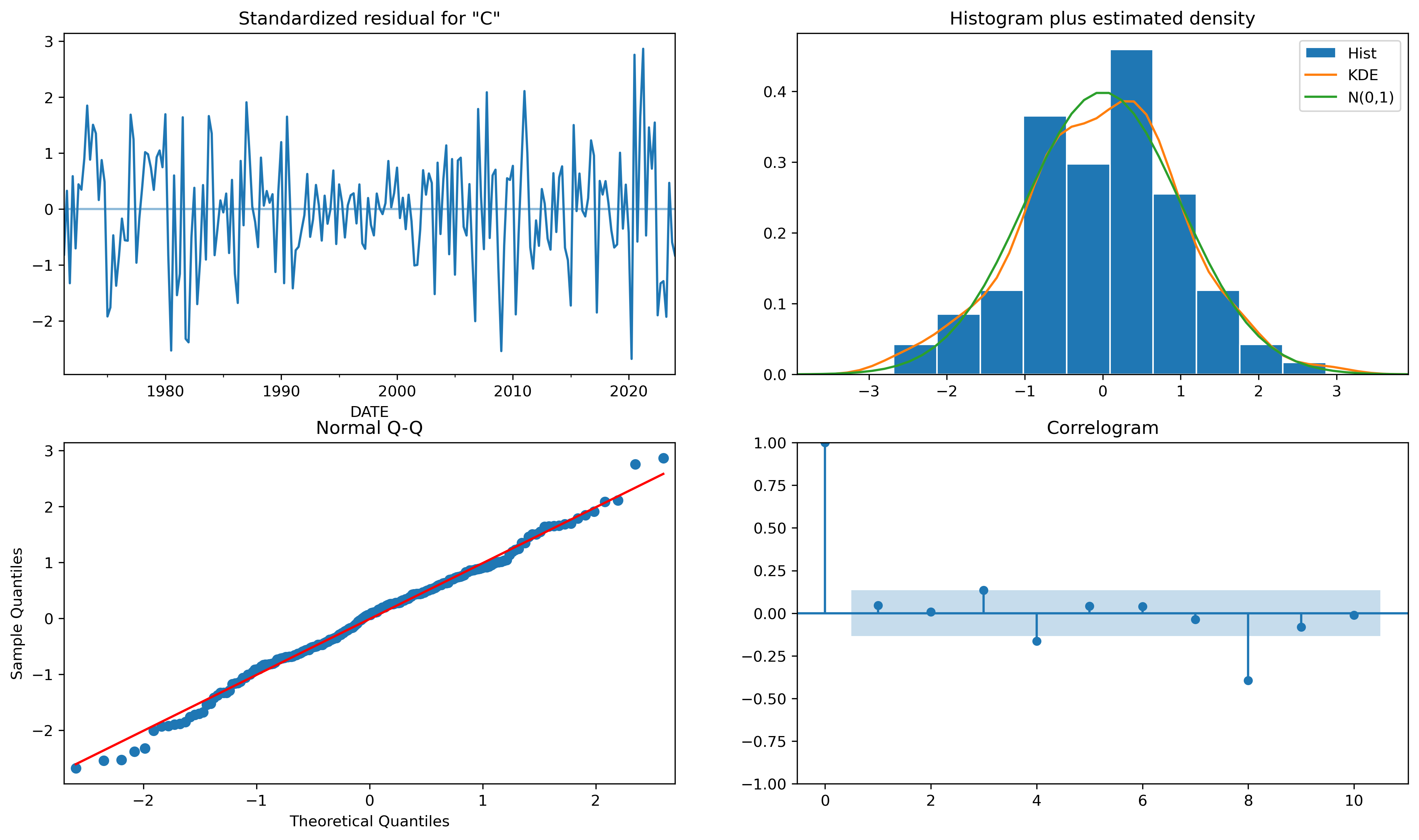
inf_results3.plot_diagnostics(figsize=(16,9));
inf_results3.forecast(4, exog=np.zeros(4))
2024-04-01    4.967205
2024-07-01    2.598361
2024-10-01   -0.654048
2025-01-01    1.485415
Freq: QS-JAN, Name: predicted_mean, dtype: float64